3  Successful Simulation

This chapter walks through a realistic simulation that successfully recovers the real spend age distribution of Litecoin (LTC) outputs. Rings are randomly generated as follows:

1. One real spend ring member is drawn from the empirical LTC distribution of ISO week 2022-10.

2. Fifteen decoys are drawn from the distribution that Monero’s “standard” wallet2 decoy selection algorithm uses.

3. A small number of “nonstandard” rings are generated from a log-triangular and a uniform decoy distribution. These rings are added to the dataset with the “standard” rings.

Applying OSPEAD techniques to the simulated ring dataset, the empirical LTC distribution of ISO week 2022-10 can be recovered. The successful estimation demonstrates that OSPEAD can recover a realistic real spend distribution from 16-member rings even in the presence of nonstandard rings.

3.1 Data generation

First, the real spend age distribution of LTC is computed. This is done for the 5th, 10th, and 15th ISO week in 2022 using this code.

Next, decoy distributions are needed. The main decoy distribution is the same as Monero’s wallet2 distribution: a log-gamma distribution with shape parameter 19.28 and rate parameter 1.61, plus a few Monero-specific adjustments. Two other decoy distributions are needed to represent nonstandard decoy selection algorithms that “third-party” Monero wallet developers may be using.

A uniform distribution, where all outputs are equally likely to be chosen, is a naive distribution that a third-party wallet developer could plausibly use. In fact, a uniform distribution was used by the standard Monero wallet in the initial months of the blockchain (Noether, Noether, and Mackenzie 2014). The second nonstandard distribution will be a log-triangular distribution, another distribution that a third-party wallet developer could plausibly use. For a period of time, the standard Monero wallet used a triangular distribution.

Important

Knowledge of the nonstandard decoy distributions is not needed for OSPEAD. In the statistical estimation, these distributions are treated as unknown. The only decoy distribution that needs to be known is the standard wallet2 distribution, which we know because it is in Monero’s open source code.

For the simulation, 300,000 rings are produced. This is approximately the number of rings that appear on the Monero blockchain in a typical week. (Note that a single transaction may have many rings.)

Three types of rings are produced:

1. Rings where one ring member is drawn from the empirical LTC distribution of ISO week 2022-10 and the remaining 15 rings members are drawn from the wallet2 log-gamma distribution. 93 percent of rings in the dataset are of this type.

2. Rings where one ring member is drawn from the empirical LTC distribution of ISO week 2022-05 and the remaining 15 rings members are drawn from a log-triangular distribution with minimum one second, maximum one year, and mode one week. 5 percent of rings in the dataset are of this type.

3. Rings where one ring member is drawn from the empirical LTC distribution of ISO week 2022-15 and the remaining 15 rings members are drawn from the a uniform distribution with minimum one second and maximum one year. 2 percent of rings in the dataset are of this type.

Notice that we use LTC distributions from different weeks. This shows that OSPEAD works even when users using the nonstandard wallet implementations do not follow the same spent output age distribution as users who use the standard wallet2 distribution.

To generate random numbers from the uniform and log-triangular distribution, the corresponding R functions (runif() and triangle::rltriangle()) are used. Random draws from the wallet2 decoy distribution and the LTC empirical distributions are accomplished by using a standard technique in probability computing. The cumulative distribution function (CDF) of each of these distributions are computed. Then, the CDFs are inverted by numerical methods to obtain the CDF inverse, also known as the quantile function. (Using numerical instead of analytical methods causes a tolerable slowdown in random number generation.) Uniform(0, 1) random numbers are transformed by the inverted CDFs to obtain random numbers with the desired distribution.

3.2 First step: Separate the wallet2 ring distribution from nonstandard rings

Distribution component “A”, associated with transactions created by wallet2, makes up 93 percent of the rings in the simulated dataset. Transactions created by wallet2 also make up the majority of transactions on the Monero blockchain. Analysis focuses on this component “A” because most transactions are in it, but also because the second step requires knowledge of the decoy selection distribution, which is known for transactions created by wallet2, but not necessarily known for transactions created by “third-party” wallet implementations.

The CDF of component “A” must be estimated. I use an estimator developed by Bonhomme, Jochmans, and Robin (2016) to accomplish the task. The BJR estimator requires the analyst to specify $K$, the number of distribution components in the dataset. In this simulation, I will set $K$ to 4, which is one more than the true number of components. I intentionally overshoot the true $K$ to demonstrate the performance of the estimator when the true $K$ is not exactly known.

The BJR estimator should take a few hours to run with the default number of threads.

3.3 Second step: Separate the real spend distribution from the wallet2 decoy distribution

Let $F_{A}(x)$ be CDF of distribution component “A”, which is a mixture distribution of $\frac{1}{16}$ parts real spend distribution $F_{A,S}(x)$ and $\frac{15}{16}$ parts wallet2 decoy distribution $F_{A,D}(x)$. The CDF of component “A” can be decomposed:

$$F_{A}(x)=\frac{1}{16}F_{A,S}(x)+\frac{15}{16}F_{A,D}(x) \qquad(3.1)$$

The BJR estimator in the first step produced an estimate of $F_{A}(x)$. The $F_{A,D}(x)$ CDF is known because it is the distribution produced by Monero’s open source decoy selection algorithm in wallet2. Equation 3.1 can be easily solved for the real spend distribution $F_{A,S}(x)$ because it is one equation in one unknown:

$$F_{A,S}(x)=16F_{A}(x)-15F_{A,D}(x) \qquad(3.2)$$

Equation 3.2 can be computed simply, but a valid CDF might not be produced because of sampling variation. Patra and Sen (2016) provides a method for adjusting the computed $F_{A,S}(x)$ to a valid CDF (i.e. weakly monotonically increasing and satisfying $\underset{x\rightarrow-\infty}{\lim}F_{A,S}(x)=0$ and $\underset{x\rightarrow\infty}{\lim}F_{A,S}(x)=1$).

3.4 Simulation results

After running the code in Section 3.6, we get the following results.

3.4.1 Mixing proportions

The mixing proportions are the share of each distribution component (A, B, C) in the dataset. Above, we set these values in the simulation to 0.93, 0.05, and 0.02, respectively. The BJR estimator can produce an estimate of these mixing proportions, based on the simulated dataset. The exact values of these estimates are not very important for OSPEAD, except that the greatest value is assumed to correspond to the wallet2-associated distribution component. Also, these results establish context for the mixing proportions results from the real Monero dataset.

The estimated mixing proportions are: 0.8898, 0.0478, 0.0191, -0.0441

Notice that the estimates are not constrained to add to 1, nor do the individual mixing proportion estimates necessarily fall between 0 and 1. What we see here is general agreement of these estimates with the mixing proportions set in the simulation parameters. The “phantom” fourth distribution component, which does not actually exist in the dataset, is estimated to have a “negative” mixing proportion.

3.4.2 Kolmogorov–Smirnov statistic

We want to know how close our estimate was to the actual LTC real spend distribution. In the next section we will view some plots, but first we will compute a numeric metric of distribution “closeness”.

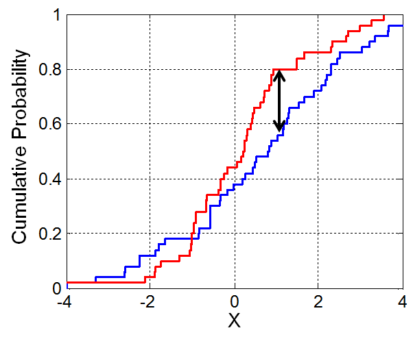
The Kolmogorov–Smirnov (KS) statistic is a common way to measure the difference between two distributions. The KS statistic is the maximum vertical distance between two CDFs. Its minimum possible value is 0 and its maximum possible value is 1. Figure 3.1 shows a visual of the KS statistic.

The KS statistic between the estimated and actual LTC real spend distribution is 0.0522.

Figure 3.1: KS Statistic. Source: Wikipedia.

3.4.3 Plots

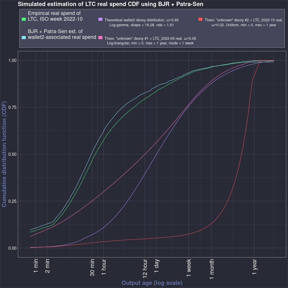
At last, we will view plots that show how accurate our estimate is. Figure 3.2 shows:

1. In green, the CDF of the real spend distribution we are trying to estimate.

2. In blue, the OSPEAD estimate of the green line.

3. In violet, the decoy selection distribution of wallet2.

4. In pink, the ring distribution of the first “unknown” decoy distribution (i.e. the log-triangular distribution) combined with the LTC real spend distribution of ISO week 2022-05.

5. In red, the ring distribution of the second “unknown” decoy distribution (i.e. the uniform distribution) combined with the LTC real spend distribution of ISO week 2022-15.

The blue line is a close, but not exact, match of the green line. The OSPEAD method estimates the real spend distribution accurately, but it is not perfect. The source of the inaccuracy is likely that ring members are not completely statistically independent, yet the BJR estimator requires independence to work flawlessly.

Figure 3.2

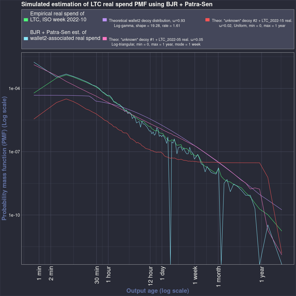
The next plot shows the probability mass functions (PMFs) associated with the CDFs plotted in Figure 3.2 . The PMFs were estimated by a simple method: computing the weighted first difference of the CDFs. The vertical axis has a log scale.

Again we see that the estimated and actual LTC real spend distributions follow each other closely. In a few places the estimated PMF is zero. This is an artifact of the Patra-Sen correction that requires the CDF to be valid. These zero-valued PMF points can be smoothed in the parametric distribution fitting step.

Figure 3.3

The next chapter, Chapter 4, begins the process to estimate the real spend age distribution of the Monero mainnet blockchain.

3.5 Is the BJR estimator necessary?

The BJR estimator is computationally expensive and consumed the majority of research and development time. Is it necessary? We can re-run the simulation, but skip the BJR step and find out.

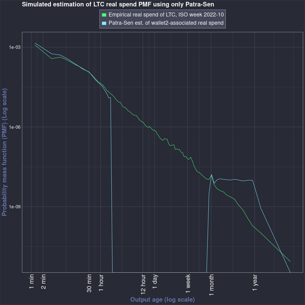
Figure 3.4 shows the results of skipping the BJR step. The estimate is quite inaccurate. It appears to bind against the non-negativity constraint of the Patra-Sen estimator. The KS statistic between this estimate and the real spend CDF is 0.2352.

Figure 3.4

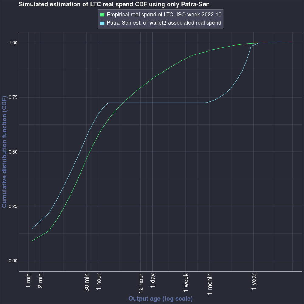
Figure 3.5 shows the PMF of the estimate that skips the BJR estimator.

Figure 3.5

3.6 Code

library(decoyanalysis)
library(ggplot2)
library(dRacula)

n.rings <- 300000

theoretical.mixing.proportions <- c(0.93, 0.05, 0.02)

threads <- 4


ltc.ecdf.2022.05 <- qs::qread("data/ltc-ecdf-2022-05.qs")
ltc.ecdf.2022.10 <- qs::qread("data/ltc-ecdf-2022-10.qs")
ltc.ecdf.2022.15 <- qs::qread("data/ltc-ecdf-2022-15.qs")

v <-  1.4
z <- 117464545
# v is the velocity of new outputs being produced on the Monero
# blockchain, in number of seconds per one new output
# z is the total number of outputs on the Monero blockchain

GAMMA_SHAPE = 19.28
GAMMA_RATE = 1.61

G <- function(x) {
  actuar::plgamma(x, shapelog = GAMMA_SHAPE, ratelog = GAMMA_RATE)
}

G_star <- function(x) {
  (0 <= x*v & x*v <= 1800) *
    (G(x*v + 1200) - G(1200) +
        ( (x*v)/(1800) ) * G(1200)
    )/G(z*v) +
    (1800 < x*v & x*v <= z*v) * G(x*v + 1200)/G(z*v) +
    (z*v < x*v) * 1
}

G_star.inv <- Vectorize(function(x) { gbutils::cdf2quantile(x, cdf = G_star) })

ltc.ecdf.2022.05.inv <- Vectorize(function(x) { gbutils::cdf2quantile(x,
  cdf = function(x) { ltc.ecdf.2022.05(x) }, lower = 0) })

ltc.ecdf.2022.10.inv <- Vectorize(function(x) { gbutils::cdf2quantile(x,
  cdf = function(x) { ltc.ecdf.2022.10(x) }, lower = 0) })

ltc.ecdf.2022.15.inv <- Vectorize(function(x) { gbutils::cdf2quantile(x,
  cdf = function(x) { ltc.ecdf.2022.15(x) }, lower = 0) })


decoy.cdfs <- list(
  function(x) { G_star(x) },
  function(x) { triangle::pltriangle(x, a = 1, b = 60*60*24*365, c = 60*60*24*7, logbase = exp(1)) },
  # a = 0 is not allowed
  function(x) { punif(x, min = 1, max = 60*60*24*365) }
)

real.spend.cdfs <- list(
  function(x) { ltc.ecdf.2022.10(x) },
  function(x) { ltc.ecdf.2022.05(x) },
  function(x) { ltc.ecdf.2022.15(x) }
)

decoy.random.draw <- list(
  function(x) { G_star.inv(runif(x)) },
  function(x) { triangle::rltriangle(x, a = 1, b = 60*60*24*365, c = 60*60*24*7, logbase = exp(1)) },
  # a = 0 is not allowed
  function(x) { runif(x, min = 1, max = 60*60*24*365) }
)

real.spend.random.draw <- list(
  function(x) { ltc.ecdf.2022.10.inv(runif(x)) },
  function(x) { ltc.ecdf.2022.05.inv(runif(x)) },
  function(x) { ltc.ecdf.2022.15.inv(runif(x)) }
)



set.seed(314)

which.component <- sample(1:3, n.rings, replace = TRUE, prob = theoretical.mixing.proportions)

which.component <- table(which.component)

ring.generation.threads <- 5
future::plan(future::multisession(workers = ring.generation.threads))

rings <- lapply(1:3, FUN = function(x) {
  cbind(
    matrix(c(future.apply::future_replicate(15, decoy.random.draw[[x]](which.component[x]))), ncol = 15),
    matrix(real.spend.random.draw[[x]](which.component[x]), ncol = 1)
  )
})

rings <- do.call(rbind, rings)

rings.untransformed <- rings

rings[rings <= 0] <- rings[rings <= 0] + 0.1
rings <- log(rings)
cdf.points <- quantile(c(rings), probs = c(0.001, (1:99)/100, 0.999))
K <- 4
II <- 10
cluster.threads <- NULL
options(future.globals.maxSize = 8000*1024^2)
future::plan(future::multisession(workers = threads))

y <- rings

print(system.time(bjr.results <- bjr(y, II = II, K = K, cdf.points = cdf.points,
  estimate.mean.sd = FALSE, basis = "Chebychev", control = list(cluster.threads = cluster.threads ))))


wallet2.dist.index <- which.max(bjr.results$mixing.proportions)
Fn.hat.value <- bjr.results$cdf$CDF[, wallet2.dist.index]
supp.points <- bjr.results$cdf$cdf
supp.points <- expm1(supp.points)
Fb <- decoy.cdfs[[1]]
M = 16
alpha <- 1/M
patra.sen.bjr.results <- patra.sen.bjr(Fn.hat.value, supp.points, Fb, alpha)


x <- bjr.results$cdf$cdf.points
x <- expm1(x)


cat("Estimated mixing proportions of distribution components:",
  paste0(round(sort(bjr.results$mixing.proportions, decreasing = TRUE), 4), collapse = ", "), "\n")

cat("Kolmogorov–Smirnov statistic (i.e. maximum distance between two CDFs) of estimated and actual LTC real spend:",
  round(max(abs(real.spend.cdfs[[1]](x) - patra.sen.bjr.results$Fs.hat)), 4), "\n")


plot.data.cdf <- data.frame(
  x = x, 
  y = c(real.spend.cdfs[[1]](x),
  patra.sen.bjr.results$Fs.hat,
  decoy.cdfs[[1]](x),
  alpha * real.spend.cdfs[[2]](x) + (1-alpha) * decoy.cdfs[[2]](x),
  alpha * real.spend.cdfs[[3]](x) + (1-alpha) * decoy.cdfs[[3]](x)
  ),
  label = as.factor(rep(1:5, each = length(x) ))
)



# NOTE: Must manualy put in the values of theoretical.mixing.proportions
# because doing it automatically is complicated.

distribution.legend.text <- c(
  expression(paste("Empirical real spend of\nLTC, ISO week 2022-10")),
  expression(paste("BJR + Patra-Sen est. of\nwallet2-associated real spend")),
  expression(atop(phantom(0), atop(paste("Theoretical wallet2 decoy distribution, ",
    omega == 0.93, ""), paste("Log-gamma, shape = 19.28, rate = 1.61")))),
  expression(atop(phantom(0), atop(paste('Theor. "unknown" decoy #1 + LTC_2022-05 real. ',
    omega == 0.05, ""), paste("Log-triangular, min = 0, max = 1 year, mode = 1 week")))),
  expression(atop(phantom(0), atop(paste('Theor. "unknown" decoy #2 + LTC_2022-15 real.'),
    paste(omega == 0.02, ", Uniform, min = 0, max = 1 year"))))
)

dracula.palette <- dracula_tibble$hex[seq_len(data.table::uniqueN(plot.data.cdf$label))]
names(dracula.palette) <- unique(plot.data.cdf$label)

if (! dir.exists("images")) { dir.create("images") }

png("images/ltc-estimation-simulation-cdf.png", width = 1000, height = 1000)

ggplot(plot.data.cdf,
  aes(x = x, y = y, colour = label)) +
  labs(title = "Simulated estimation of LTC real spend CDF using BJR + Patra-Sen",
    y = "Cumulative distribution function (CDF)",
    x = "Output age (log scale)") +
  geom_line() +
  scale_x_log10(
    guide = guide_axis(angle = 90),
    breaks = c(1, 10, 60, 60*2, 60*30, 60^2, 60^2*12, 60^2*24, 60^2*24*7, 60^2*24*28, 60^2*24*365),
    labels = c("1 sec", "10 sec", "1 min", "2 min", "30 min", "1 hour", "12 hour", "1 day", "1 week", "1 month", "1 year")) +
  # scale_colour_brewer(palette = "Dark2") +
  theme_dracula() +
  theme(
    legend.position = "top",
    legend.title = element_blank(),
    panel.border = element_rect(color = "white", fill = NA),
    plot.title = element_text(size = 20),
    legend.text = element_text(size = 18),
    axis.text.y = element_text(size = 15),
    axis.text.x = element_text(size = 20),
    axis.title.y = element_text(size = 20),
    axis.title.x = element_text(size = 20)
    ) + 
  scale_colour_manual(values = dracula.palette, name = '', 
    labels = distribution.legend.text, guide = guide_legend(nrow = 2, override.aes = list(linewidth = 5)))
# The order of the themes() matter. Must have theme_dracula() first.

dev.off()


plot.data.pmf <- data.frame(
  x = x[-1], 
  y = c(
    diff(real.spend.cdfs[[1]](x)) / diff(x),
    diff(patra.sen.bjr.results$Fs.hat) / diff(x),
    diff(decoy.cdfs[[1]](x)) / diff(x),
    diff(alpha * real.spend.cdfs[[2]](x) + (1-alpha) * decoy.cdfs[[2]](x)) / diff(x),
    diff(alpha * real.spend.cdfs[[3]](x) + (1-alpha) * decoy.cdfs[[3]](x)) / diff(x)
  ),
  label = as.factor(rep(1:5, each = length(x) - 1 ))
)



png("images/ltc-estimation-simulation-pmf.png", width = 1000, height = 1000)

ggplot(plot.data.pmf,
  aes(x = x, y = y, colour = label)) +
  labs(title = "Simulated estimation of LTC real spend PMF using BJR + Patra-Sen",
    y = "Probability mass function (PMF) (Log scale)",
    x = "Output age (log scale)") +
  geom_line() +
 # coord_cartesian(ylim = c(0.00000000001, 0.1)) +
  scale_y_log10() + 
  scale_x_log10(
    guide = guide_axis(angle = 90),
    breaks = c(1, 10, 60, 60*2, 60*30, 60^2, 60^2*12, 60^2*24, 60^2*24*7, 60^2*24*28, 60^2*24*365),
    labels = c("1 sec", "10 sec", "1 min", "2 min", "30 min", "1 hour", "12 hour", "1 day", "1 week", "1 month", "1 year")) +
  # scale_colour_brewer(palette = "Dark2") +
  theme_dracula() +
  theme(
    legend.position = "top",
    legend.title = element_blank(),
    panel.border = element_rect(color = "white", fill = NA),
    plot.title = element_text(size = 20),
    legend.text = element_text(size = 18),
    axis.text.y = element_text(size = 15),
    axis.text.x = element_text(size = 20),
    axis.title.y = element_text(size = 20),
    axis.title.x = element_text(size = 20)
  ) + 
  scale_colour_manual(values = dracula.palette, name = '', 
    labels = distribution.legend.text, guide = guide_legend(nrow = 2, override.aes = list(linewidth = 5)))
# The order of the themes() matter. Must have theme_dracula() first.

dev.off()




# Alternative LTC estimation with only Patra-Sen


rings.ecdf <- ecdf(c(rings.untransformed))
supp.points <- knots(rings.ecdf)[floor(seq(1, length(knots(rings.ecdf)), length.out = 101))]
Fn.hat.value <- rings.ecdf(supp.points)

Fb <- decoy.cdfs[[1]]
M = 16
alpha <- 1/M
patra.sen.bjr.results <- patra.sen.bjr(Fn.hat.value, supp.points, Fb, alpha)

x <- supp.points

cat("Kolmogorov–Smirnov statistic (i.e. maximum distance between two CDFs) of estimated and actual LTC real spend:",
  round(max(abs(real.spend.cdfs[[1]](x) - patra.sen.bjr.results$Fs.hat)), 4), "\n")



plot.data.cdf <- data.frame(
  x = x, 
  y = c(real.spend.cdfs[[1]](x),
    patra.sen.bjr.results$Fs.hat
  ),
  label = as.factor(rep(1:2, each = length(x) ))
)


# NOTE: Must manualy put in the values of theoretical.mixing.proportions
# because doing it automatically is complicated.

distribution.legend.text <- c(
  expression(paste("Empirical real spend of LTC, ISO week 2022-10")),
  expression(paste("Patra-Sen est. of wallet2-associated real spend")),
  expression(atop(phantom(0), atop(paste("Theoretical wallet2 decoy distribution, ",
    omega == 0.93, ""), paste("Log-gamma, shape = 19.28, rate = 1.61")))),
  expression(atop(phantom(0), atop(paste('Theor. "unknown" decoy #1 + LTC_2022-05 real. ',
    omega == 0.05, ""), paste("Log-triangular, min = 0, max = 1 year, mode = 1 week")))),
  expression(atop(phantom(0), atop(paste('Theor. "unknown" decoy #2 + LTC_2022-15 real.'),
    paste(omega == 0.02, ", Uniform, min = 0, max = 1 year"))))
)

dracula.palette <- dracula_tibble$hex[seq_len(data.table::uniqueN(plot.data.cdf$label))]
names(dracula.palette) <- unique(plot.data.cdf$label)

if (! dir.exists("images")) { dir.create("images") }

png("images/ltc-estimation-simulation-cdf-only-patra-sen.png", width = 1000, height = 1000)

ggplot(plot.data.cdf,
  aes(x = x, y = y, colour = label)) +
  labs(title = "Simulated estimation of LTC real spend CDF using only Patra-Sen",
    y = "Cumulative distribution function (CDF)",
    x = "Output age (log scale)") +
  geom_line() +
  scale_x_log10(
    guide = guide_axis(angle = 90),
    breaks = c(1, 10, 60, 60*2, 60*30, 60^2, 60^2*12, 60^2*24, 60^2*24*7, 60^2*24*28, 60^2*24*365),
    labels = c("1 sec", "10 sec", "1 min", "2 min", "30 min", "1 hour", "12 hour", "1 day", "1 week", "1 month", "1 year")) +
  # scale_colour_brewer(palette = "Dark2") +
  theme_dracula() +
  theme(
    legend.position = "top",
    legend.title = element_blank(),
    panel.border = element_rect(color = "white", fill = NA),
    plot.title = element_text(size = 20),
    legend.text = element_text(size = 18),
    axis.text.y = element_text(size = 15),
    axis.text.x = element_text(size = 20),
    axis.title.y = element_text(size = 20),
    axis.title.x = element_text(size = 20)
  ) + 
  scale_colour_manual(values = dracula.palette, name = '', 
    labels = distribution.legend.text, guide = guide_legend(nrow = 2, override.aes = list(linewidth = 5)))
# The order of the themes() matter. Must have theme_dracula() first.

dev.off()


plot.data.pmf <- data.frame(
  x = x[-1], 
  y = c(
    diff(real.spend.cdfs[[1]](x)) / diff(x),
    diff(patra.sen.bjr.results$Fs.hat) / diff(x)
  ),
  label = as.factor(rep(1:2, each = length(x) - 1 ))
)



png("images/ltc-estimation-simulation-pmf-only-patra-sen.png", width = 1000, height = 1000)

ggplot(plot.data.pmf,
  aes(x = x, y = y, colour = label)) +
  labs(title = "Simulated estimation of LTC real spend PMF using only Patra-Sen",
    y = "Probability mass function (PMF) (Log scale)",
    x = "Output age (log scale)") +
  geom_line() +
  # coord_cartesian(ylim = c(0.00000000001, 0.1)) +
  scale_y_log10() + 
  scale_x_log10(
    guide = guide_axis(angle = 90),
    breaks = c(1, 10, 60, 60*2, 60*30, 60^2, 60^2*12, 60^2*24, 60^2*24*7, 60^2*24*28, 60^2*24*365),
    labels = c("1 sec", "10 sec", "1 min", "2 min", "30 min", "1 hour", "12 hour", "1 day", "1 week", "1 month", "1 year")) +
  # scale_colour_brewer(palette = "Dark2") +
  theme_dracula() +
  theme(
    legend.position = "top",
    legend.title = element_blank(),
    panel.border = element_rect(color = "white", fill = NA),
    plot.title = element_text(size = 20),
    legend.text = element_text(size = 18),
    axis.text.y = element_text(size = 15),
    axis.text.x = element_text(size = 20),
    axis.title.y = element_text(size = 20),
    axis.title.x = element_text(size = 20)
  ) + 
  scale_colour_manual(values = dracula.palette, name = '', 
    labels = distribution.legend.text, guide = guide_legend(nrow = 2, override.aes = list(linewidth = 5)))
# The order of the themes() matter. Must have theme_dracula() first.

dev.off()

Bonhomme, Stéphane, Koen Jochmans, and Jean-Marc Robin. 2016. “Non-Parametric Estimation of Finite Mixtures from Repeated Measurements.” Journal of the Royal Statistical Society. Series B (Statistical Methodology) 78 (1): 211–29. http://www.jstor.org/stable/24775334.

Noether, Surae, Sarang Noether, and Adam Mackenzie. 2014. “A Note on Chain Reactions in Traceability in CryptoNote 2.0.” Research Bulletin. https://www.getmonero.org/resources/research-lab/pubs/MRL-0001.pdf.

Patra, Rohit Kumar, and Bodhisattva Sen. 2016. “Estimation of a Two-Component Mixture Model with Applications to Multiple Testing.” Journal of the Royal Statistical Society. Series B (Statistical Methodology) 78 (4): 869–93. http://www.jstor.org/stable/24775367.