11  Real Spend Visualization

This chapter plots the results of the real spend distribution estimation, week-by-week.

11.1 Summary statistics

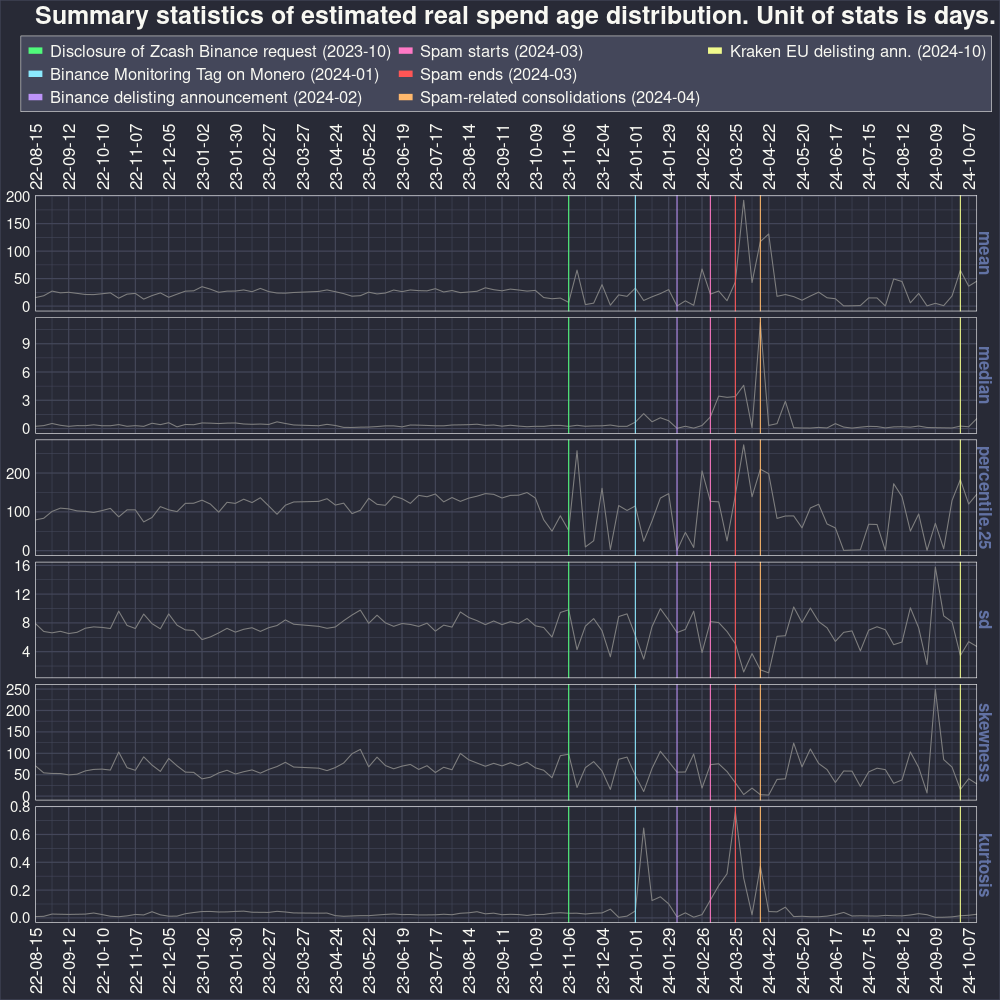
Figure 11.1 plots mean, median, 25th percentile, standard deviation, skewness, and kurtosis. Several events are indicated with colored vertical lines. The summary statistics were relatively stable until the first indicated event, the announcement of the Zcash community forum that Binance requested a protocol change: “A representative from Binance’s listing team recently approached the Zcash core teams about a way to prevent users from sending ZEC from a shielded address to a transparent address on the Binance exchange.” Thereafter, the summary statistics are more volatile week-to-week. Uncertainty in the exchange rate market may have large effects on the real spend age distribution as speculative inflows and outflows from centralized exchanges change from week to week. The share of Monero transactions related to centralized exchanges is unknown, but an estimated 75 percent of bitcoin transactions are inflows or outflows from exchange-like entities (Makarov and Schoar 2021).

During the March 2024 suspected spam attack, the median age of spent outputs increased. The age distribution shifted in the opposite direction during the earlier 2021 suspected spam wave (Krawiec-Thayer et al. 2021). The shift towards older outputs could be explained by the spammer’s spending script and/or changes in normal user behavior because of a congested txpool. The median age peaked to 11 days during the suspected spam-related consolidation transactions in April 2024. Probably, the spammer was consolidating outputs that were created during the spam a few weeks prior.

Figure 11.1

11.2 Mixing proportions

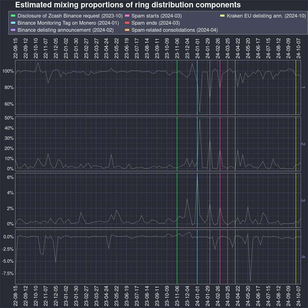
Figure 11.2 plots the mixing proportions of the distribution components estimated by the BJR estimator. The $i$th mixing proportion in each week does not necessarily refer to the same distribution week-to-week. (This is due to the labeling identification problem of mixture distributions.) The mixing proportions are simply sorted from highest to lowest.

Large deviations in the mixing proportions are observed during significant exogenous events like delisting announcements and spam. It is likely that the BJR estimator split the single wallet2-associated ring distribution into two distributions during those events because the real spend distribution itself split into users (or spammers) who were reacting to the event and those who did not react. Another possibility, though unlikely, is that users who use nonstandard wallets were more likely to transact during these events. The next chapter will discuss how these events can be handled for the overall parametric fitting step.

Figure 11.2

11.3 Animations

11.3.1 PMF, non-log Y axis

Below is an animation of the probability mass function (PMF) of the estimated real spend distribution of the first 48 hours of the distribution. Each week is one frame. The animation can be controlled by clicking buttons on the panel below the animation.

11.3.2 PMF, log Y axis

Below is the same animation, but with a log Y axis.

11.3.3 CDF

Below is an animation of the cumulative distribution function (CDF) of the estimated real spend distribution of the first 48 hours of the distribution.

11.4 Code

This code can be run in a new R session

library(ggplot2)
library(dRacula)
library(animation)

results.dir <- "results"

results.dir.run <- paste0(results.dir, "/results-01/")


nonparametric.real.spend <- qs::qread(file = paste0(results.dir.run, "nonparametric-real-spend.qs"))

nonparametric.real.spend <- nonparametric.real.spend$rucknium


# Static timeline plots


dark.mode <- TRUE

if (dark.mode) {
  brewed.cols <- dracula_tibble$hex
} else {
  brewed.cols <- RColorBrewer::brewer.pal(8, "Accent")[-4]
}



ISOweek2date.convert <- function(x) {
  x <- gsub("[.]qs", "", x)
  x <- strsplit(x, "-")
  x <- sapply(x, FUN = function(z) { paste0(z[1], "-W", z[2], "-1") } )
  ISOweek::ISOweek2date(x)
}




vert.lines <- data.frame(
  week = ISOweek2date.convert(c("2023-45", "2024-01", "2024-06", "2024-10",
    "2024-13", "2024-16", "2024-40")),
  week.iso = c("2023-45", "2024-01", "2024-06", "2024-10",
    "2024-13", "2024-16", "2024-40"),
  label = c("Disclosure of Zcash Binance request (2023-10)", "Binance Monitoring Tag on Monero (2024-01)",
    "Binance delisting announcement (2024-02)", "Spam starts (2024-03)", "Spam ends (2024-03)",
    "Spam-related consolidations (2024-04)", "Kraken EU delisting ann. (2024-10)"),
  color = brewed.cols
)
  # 1) Nov 9 https://forum.zcashcommunity.com/t/important-potential-binance-delisting/45954
  # 2) https://monero.observer/binance-marks-monero-potential-delisting/
  # 3) https://monero.observer/binance-decides-to-finally-delist-monero-20-february-2024/
  # 4) https://github.com/Rucknium/misc-research/blob/main/Monero-Black-Marble-Flood/pdf/monero-black-marble-flood.pdf
  # 5) https://github.com/Rucknium/misc-research/blob/main/Monero-Black-Marble-Flood/pdf/monero-black-marble-flood.pdf
  # 6) Suspected spam-related consolidation transactions April 16 and 17
  #    https://libera.monerologs.net/monero-research-lab/20240417#c366338
  # 7) https://monero.observer/kraken-to-delist-monero-european-economic-area-31-october-2024/


est.summary.stats <- reshape(nonparametric.real.spend$summary.stats,
  dir = "long", idvar = "week",
  varying = setdiff(names(nonparametric.real.spend$summary.stats), "week"), v.names = "y")  
names(est.summary.stats) <- c("week", "stat", "y")
# est.summary.stats$stat <- factor(est.summary.stats$stat, labels = attr(est.summary.stats, "reshapeLong")$varying$y)
est.summary.stats$stat <- factor(est.summary.stats$stat,
  labels = c("mean", "median", "percentile.25", "sd", "skewness", "kurtosis"))
# Manually specify to control the order
est.summary.stats$week <- ISOweek2date.convert(est.summary.stats$week)


est.summary.stats$dummy.color <- factor(rep(NA, nrow(est.summary.stats)),
  levels = brewed.cols, labels = brewed.cols)


png("images/real-spend-summary-stats-dark-mode.png", width = 1000, height = 1000)

gg <- ggplot(data = est.summary.stats, aes(week, y, group = stat, color = dummy.color)) +
  labs(title = "Summary statistics of estimated real spend age distribution. Unit of stats is days.") + 
  geom_line(show.legend = TRUE) +
  # geom_vline(aes(xintercept = week, color = color), data = vert.lines, linetype = 2) +
  # This format above doesn't work. Must specify them individually:
  geom_vline(xintercept = vert.lines$week[1], color = vert.lines$color[1], linetype = 1) +
  geom_vline(xintercept = vert.lines$week[2], color = vert.lines$color[2], linetype = 1) +
  geom_vline(xintercept = vert.lines$week[3], color = vert.lines$color[3], linetype = 1) +
  geom_vline(xintercept = vert.lines$week[4], color = vert.lines$color[4], linetype = 1) +
  geom_vline(xintercept = vert.lines$week[5], color = vert.lines$color[5], linetype = 1) +
  geom_vline(xintercept = vert.lines$week[6], color = vert.lines$color[6], linetype = 1) +
  geom_vline(xintercept = vert.lines$week[7], color = vert.lines$color[7], linetype = 1) +
  scale_x_date(date_breaks = "4 week", guide = guide_axis(angle = 90),
    date_labels = "%y-%m-%d", sec.axis = dup_axis(), expand = c(0, 0)) +
  facet_grid(rows = vars(stat), scales = "free") +
  scale_color_manual(limits = vert.lines$label, values = vert.lines$color, name = NULL,
    drop = FALSE, guide = guide_legend(nrow = 3, byrow = FALSE, override.aes = list(linewidth = 3)))


if (dark.mode) {
  gg +
    theme_dracula() +
    theme(
      legend.position = "top",
      axis.title.y = element_blank(),
      axis.title.x = element_blank(),
      plot.title = element_text(size = 25),
      legend.text = element_text(size = 16.5),
      axis.text.y = element_text(size = 15),
      axis.text.x = element_text(size = 17),
      strip.text = element_text(size = 17),
      panel.border = element_rect(color = "white", fill = NA)
    )
} else {
  gg +
    theme(
      legend.position = "top",
      axis.title.y = element_blank(),
      axis.title.x = element_blank(),
      plot.title = element_text(size = 25),
      legend.text = element_text(size = 16.5),
      axis.text.y = element_text(size = 15),
      axis.text.x = element_text(size = 17),
      strip.text = element_text(size = 17),
      panel.border = element_rect(color = "white", fill = NA)
    )
  # theme() must go after theme_dracula()
}


dev.off()






est.mixing.proportions <- reshape(nonparametric.real.spend$mixing.proportions,
  dir = "long", idvar = "week",
  varying = setdiff(names(nonparametric.real.spend$mixing.proportions), "week"), v.names = "y")  
names(est.mixing.proportions) <- c("week", "component", "y")

est.mixing.proportions$week <- ISOweek2date.convert(est.mixing.proportions$week)



est.mixing.proportions$dummy.color <- factor(rep(NA, nrow(est.mixing.proportions)),
  levels = brewed.cols, labels = brewed.cols)




png("images/mixing-proportions-dark-mode.png", width = 1000, height = 1000)

gg <- ggplot(data = est.mixing.proportions, aes(week, y, group = component, color = dummy.color)) +
  labs(title = "Estimated mixing proportions of ring distribution components") + 
  geom_line(show.legend = TRUE) +
  # geom_vline(aes(xintercept = week, color = color), data = vert.lines, linetype = 2) +
  # This format above doesn't work. Must specify them individually:
  geom_vline(xintercept = vert.lines$week[1], color = vert.lines$color[1], linetype = 1) +
  geom_vline(xintercept = vert.lines$week[2], color = vert.lines$color[2], linetype = 1) +
  geom_vline(xintercept = vert.lines$week[3], color = vert.lines$color[3], linetype = 1) +
  geom_vline(xintercept = vert.lines$week[4], color = vert.lines$color[4], linetype = 1) +
  geom_vline(xintercept = vert.lines$week[5], color = vert.lines$color[5], linetype = 1) +
  geom_vline(xintercept = vert.lines$week[6], color = vert.lines$color[6], linetype = 1) +
  geom_vline(xintercept = vert.lines$week[7], color = vert.lines$color[7], linetype = 1) +
  scale_x_date(date_breaks = "4 week", guide = guide_axis(angle = 90),
    date_labels = "%y-%m-%d", sec.axis = dup_axis(), expand = c(0, 0)) +
  scale_y_continuous(labels = scales::percent) +
  facet_grid(rows = vars(component), scales = "free") +
  scale_color_manual(limits = vert.lines$label, values = vert.lines$color, name = NULL,
    drop = FALSE, guide = guide_legend(nrow = 3, byrow = FALSE, override.aes = list(linewidth = 3)))


if (dark.mode) {
  gg +
    theme_dracula() +
    theme(
      legend.position = "top",
      axis.title.y = element_blank(),
      axis.title.x = element_blank(),
      plot.title = element_text(size = 25),
      legend.text = element_text(size = 16.5),
      axis.text.y = element_text(size = 15),
      axis.text.x = element_text(size = 17),
      strip.text = element_text(size = 17),
      panel.border = element_rect(color = "white", fill = NA)
    )
} else {
  gg +
    theme(
      legend.position = "top",
      axis.title.y = element_blank(),
      axis.title.x = element_blank(),
      plot.title = element_text(size = 25),
      legend.text = element_text(size = 16.5),
      axis.text.y = element_text(size = 15),
      axis.text.x = element_text(size = 17),
      strip.text = element_text(size = 17),
      panel.border = element_rect(color = "white", fill = NA)
    )
  # theme() must go after theme_dracula()
}


dev.off()





# Animation plots




weekly.real.spend.cdfs <- nonparametric.real.spend$weekly.real.spend.cdfs

all.weeks.weighted.v.mean <- nonparametric.real.spend$all.weeks.weighted.v.mean

weighted.v.mean <- mean(all.weeks.weighted.v.mean)

support.max <- nonparametric.real.spend$support.max

days.unit <- weighted.v.mean/(60^2*24)
minutes.unit <- weighted.v.mean/(60)



GAMMA_SHAPE = 19.28
GAMMA_RATE = 1.61

G <- function(x) {
  actuar::plgamma(x, shapelog = GAMMA_SHAPE, ratelog = GAMMA_RATE)
}

G_star <- function(x) {
  (0 <= x*v & x*v <= 1800) *
    (G(x*v + 1200) - G(1200) +
        ( (x*v)/(1800) ) * G(1200)
    )/G(z*v) +
    (1800 < x*v & x*v <= z*v) * G(x*v + 1200)/G(z*v) +
    (z*v < x*v) * 1
}




support.viz <- 1:ceiling(60*48/minutes.unit)


empirical.cdf <- weekly.real.spend.cdfs

year.week.range <- sort(names(weekly.real.spend.cdfs))

weekly.historical.length <- 52/2

col.palette <- viridis::magma(weekly.historical.length)

ani.options(interval = 1, ani.height = 1000, ani.width = 1000, verbose = FALSE)

# PMF

for (log.y in c(FALSE, TRUE)) {
  
  saveHTML({
    
    for (i in seq_along(year.week.range) ) {
      
      subset.seq <- 1:i
      subset.seq <- subset.seq[max(1, i - weekly.historical.length + 1):max(subset.seq)]
      col.palette.subset <- col.palette[max(1, weekly.historical.length - i + 1):weekly.historical.length]
      col.palette.subset[length(col.palette.subset)] <- "green"
      
      year.week.range.subset <- year.week.range[subset.seq]
      
      par(bg = 'black', fg = 'white', cex = 2)
      
      plot(1,
        main = paste0("PMF of estimated real spend age,\nby week of transaction"),
        sub = paste0("ISO week ", gsub(".qs", "", year.week.range[i]), " (Week starting ",
          # as.Date(paste0(year.week.range[i], "-1"), "%Y-%U.qs-%u"), ")"),
          ISOweek2date.convert(year.week.range[i]), ")" ),
        ylab = ifelse(log.y, "PMF (log scale)", "PMF"), xlab = "Age of spent output (log scale)",
        col.lab = "white", col.axis = "white", col.main = "white", col.sub = "white",
        col = "transparent", log = ifelse(log.y, "xy", "x"),
        xlim = (range(support.viz) + 1)* minutes.unit,
        ylim = ifelse(rep(log.y, 2), c(.0000002, 0.01), c(0, 0.005)),
        xaxt = "n", yaxs = "i")
      
      for ( j in seq_along(subset.seq)) {
        lines(
          (support.viz[-length(support.viz)][-1]) * minutes.unit,
          diff(empirical.cdf[[ year.week.range.subset[j] ]]( c(support.viz[-length(support.viz)] + 1))),
          col = col.palette.subset[j],
          lwd = ifelse(j == length(subset.seq), 2, 0.5)
        )
      }
      
      v <- all.weeks.weighted.v.mean[ year.week.range[i] ]
      z <- support.max
      
      status.quo.decoy <- diff(G_star(as.numeric(support.viz)))
      
      lines(support.viz[-1] * minutes.unit, status.quo.decoy, col = "red", lwd = 2)
      
      cat(i, " ")
      
      legend("topright", legend = c("Decoy status quo"), fill = c("red"))
      
      axis(side = 1, at = c(1/6, 1, 10, 60, 60*12, 60*48),
        labels = c("10 sec", "1 min", "10 min", "1 hour", "12 hrs", "48 hrs"),
        col.axis = "white", las = 2, cex.axis = 0.8)
      
      axis(side = 4, col.axis = "white")
      
      if (gsub(".qs", "", year.week.range[i]) %in% vert.lines$week.iso) {
        event.label <- vert.lines$label[vert.lines$week.iso == gsub(".qs", "", year.week.range[i]) ]
        event.label <- paste0("Event: ", gsub(" [(].*[)]", "", event.label))
        # y.event.pos <- ifelse(rep(log.y, 2), c(.0000002, 0.01), c(0, 0.005))
        mtext(event.label, side = 3, line = -4, adj = 0.98, col = "white", cex = 1.5)
      }
      
      # abline(h = 0, lty = 2)
      
      
    }
  }, 
    img.name = ifelse(log.y, "real-spend-pmf-by-week-y-log", "real-spend-pmf-by-week-not-y-log"),
    navigator = TRUE,
    htmlfile = ifelse(log.y, "real-spend-pmf-by-week-y-log.html", "real-spend-pmf-by-week-not-y-log.html"),
    # htmlfile has no effect for the Quarto book since only pieces of the file are used.
    autobrowse = FALSE
    )
  

  
}




# CDF


for (log.y in c(FALSE)) {
  
  saveHTML({
    
    for (i in seq_along(year.week.range) ) {
      
      subset.seq <- 1:i
      subset.seq <- subset.seq[max(1, i - weekly.historical.length + 1):max(subset.seq)]
      col.palette.subset <- col.palette[max(1, weekly.historical.length - i + 1):weekly.historical.length]
      col.palette.subset[length(col.palette.subset)] <- "green"
      
      year.week.range.subset <- year.week.range[subset.seq]
      
      par(bg = 'black', fg = 'white', cex = 2)
      
      plot(1,
        main = paste0("CDF of estimated real spend age,\nby week of transaction"),
        sub = paste0("ISO week ", gsub(".qs", "", year.week.range[i]), " (Week starting ",
          # as.Date(paste0(year.week.range[i], "-1"), "%Y-%U.qs-%u"), ")"),
          ISOweek2date.convert(year.week.range[i]), ")" ),
        ylab = ifelse(log.y, "CDF (log scale)", "CDF"), xlab = "Age of spent output (log scale)",
        col.lab = "white", col.axis = "white", col.main = "white", col.sub = "white",
        col = "transparent", log = ifelse(log.y, "xy", "x"),
        xlim = (range(support.viz) + 1)* minutes.unit,
        ylim = ifelse(rep(log.y, 2), c(.0000002, 1), c(0, 1)),
        xaxt = "n", yaxt = "n")
      
      for ( j in seq_along(subset.seq)) {
        lines((support.viz[-length(support.viz)]) * minutes.unit,
          empirical.cdf[[ year.week.range.subset[j] ]]( c(support.viz[-length(support.viz)] + 1)),
          col = col.palette.subset[j],
          lwd = ifelse(j == length(subset.seq), 2, 0.5)
        )
      }
      
      v <- all.weeks.weighted.v.mean[ year.week.range[i] ]
      z <- support.max
      
      status.quo.decoy <- G_star(as.numeric(support.viz))
      
      lines(support.viz * minutes.unit, status.quo.decoy, col = "red", lwd = 2)
      
      cat(i, " ")
      
      legend("topleft", legend = c("Decoy status quo"), fill = c("red"))
      
      axis(side = 1, at = c(1/6, 1, 10, 60, 60*12, 60*48),
        labels = c("10 sec", "1 min", "10 min", "1 hour", "12 hrs", "48 hrs"),
        col.axis = "white", las = 2, cex.axis = 0.8)
      
      axis(side = 2, at = seq(0, 1, by = 0.1), col.axis = "white", cex.axis = 0.8, las = 1)
      axis(side = 4, at = seq(0, 1, by = 0.1), col.axis = "white", cex.axis = 0.8, las = 1)
      
      if (gsub(".qs", "", year.week.range[i]) %in% vert.lines$week.iso) {
        event.label <- vert.lines$label[vert.lines$week.iso == gsub(".qs", "", year.week.range[i]) ]
        event.label <- paste0("Event: ", gsub(" [(].*[)]", "", event.label))
        # y.event.pos <- ifelse(rep(log.y, 2), c(.0000002, 0.01), c(0, 0.005))
        mtext(event.label, side = 3, line = -4, adj = 0.02, col = "white", cex = 1.5)
      }
      
      # abline(h = 0, lty = 2)
      
      
    }
  }, 
    img.name = ifelse(log.y, "real-spend-cdf-by-week-y-log", "real-spend-cdf-by-week-not-y-log"),
    navigator = TRUE,
    htmlfile = ifelse(log.y, "real-spend-cdf-by-week-y-log.html", "real-spend-cdf-by-week-not-y-log.html"),
    # htmlfile has no effect for the Quarto book since only pieces of the file are used.
    autobrowse = FALSE
    )
  

}

Krawiec-Thayer, Mitchell P., Neptune, Rucknium, Jberman, and Carrington. 2021. “Fingerprinting a Flood: Forensic Statistical Analysis of the Mid-2021 Monero Transaction Volume Anomaly.” https://mitchellpkt.medium.com/fingerprinting-a-flood-forensic-statistical-analysis-of-the-mid-2021-monero-transaction-volume-a19cbf41ce60.

Makarov, Igor, and Antoinette Schoar. 2021. “Blockchain Analysis of the Bitcoin Market.” Working Paper 29396. Working Paper Series. National Bureau of Economic Research. https://doi.org/10.3386/w29396.