13  Performance Evaluation

With the parametric fit done in Chapter 12 , we can evaluate how well the parametric distributions would protect users against the MAP Decoder attack.

With ring size 16, the minimum possible attack success probability is $1/16=6.25\%$.

13.1 Attack success probability

Table 13.1 shows the top six best distributions, the average attack success probability computed from Equation 12.1 , and the fitted parameter values. Note that some of the distributions have the same names for parameters, but they have different meanings for each parametric distribution. Consult the sources in Section 12.2 and the documentation for the distributions’ R implementations in Section 12.4 for their meanings.

The lowest attack success probability is achieved by Log-GB2, the log transformation of the generalized beta distribution of the second kind. If Monero’s default decoy selection algorithm were Log-GB2 with the specified parameter values, an adversary applying the MAP decoder attack would have successfully guessed the real spend in 7.6 percent of rings, on average, since the August 2022 hard fork. That corresponds to an effective ring size of 13.2.

The last row of Table 13.1 shows the estimated average attack success probability that an adversary can achieve against real Monero users who were using the default wallet2 decoy selection algorithm, since the August 2022 hard fork: 23.5 percent. This corresponds to an effective ring size of 4.2.

Table 13.1: Attack success probability with fitted parametric decoy distributions

Decoy distribution	Attack success probability	Param 1	Param 2	Param 3	Param 4
Log-GB2	7.590%	shape1 = 4.462	scale = 20.62	shape2 = 0.5553	shape3 = 7.957
Log-GEV	7.730%	location = 8.382	scale = 3.851	shape = -0.3404
RPLN	7.746%	shape2 = 6.684	meanlog = 9.725	sdlog = 3.964
GB2	7.794%	shape1 = 0.1282	scale = 4753	shape2 = 8.582	shape3 = 7.179
Log-F	8.212%	df1 = 1.678	df2 = 9.067e+06	ncp = 17.06
Log-Gamma	8.470%	shape = 4.315	rate = 0.3751
Decoy status quo	23.540%	shape = 19.28	rate = 1.61

13.2 Visualizations of fitted distributions

Figure 13.1 compares the probability mass functions of the top three fitted decoy distributions, the status quo decoy distribution, and the real spend distribution. I included the CDF of the real spend on the bottom panel because PMFs on a log scale can appear misleading.

Outputs in the first two minutes would usually be included in a single block. Therefore, variations in the probability mass within those two minutes are not very meaningful.

The figure shows that the probability mass of the status quo decoy distribution is much lower than the real spend. Therefore, the status quo decoy distribution is not doing a good job of protecting the privacy of users who spend young outputs.

Figure 13.1

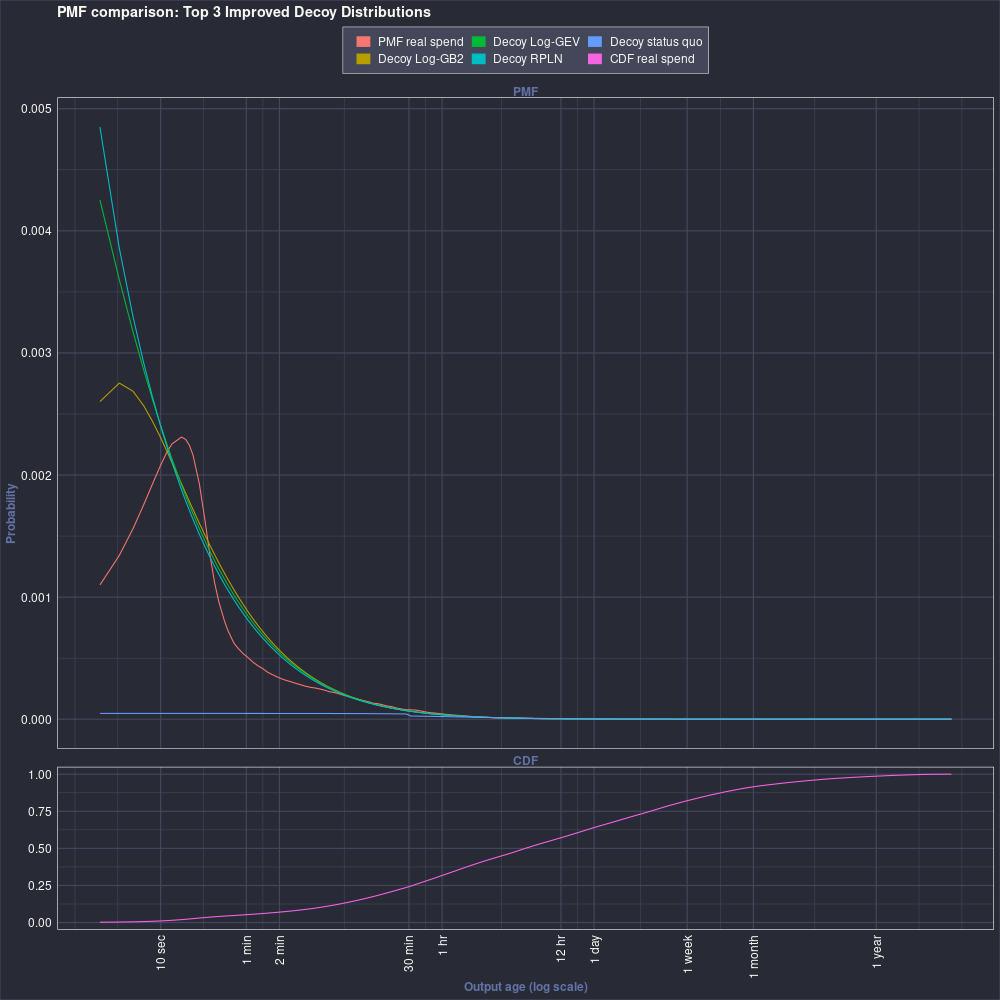
Figure 13.2 shows the PMFs of the top 4-6 distributions from Table 13.1 .

Figure 13.2

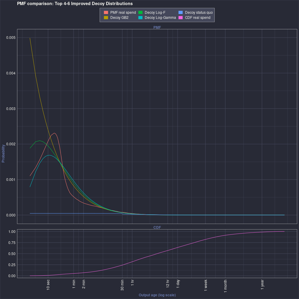
Figure 13.3 is the same plot as Figure 13.1 , except the vertical axis is log scale. The log scale makes it easier to see the differences in the PMFs for older outputs.

Figure 13.3

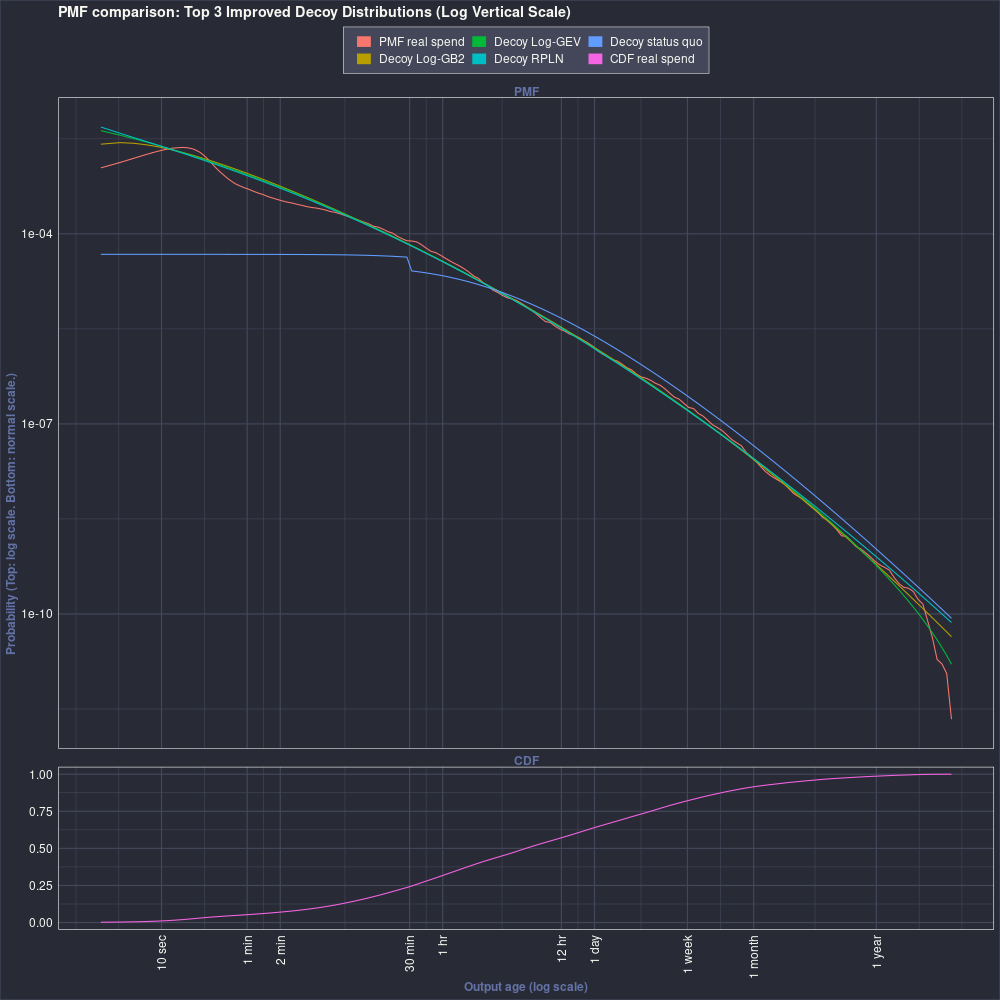
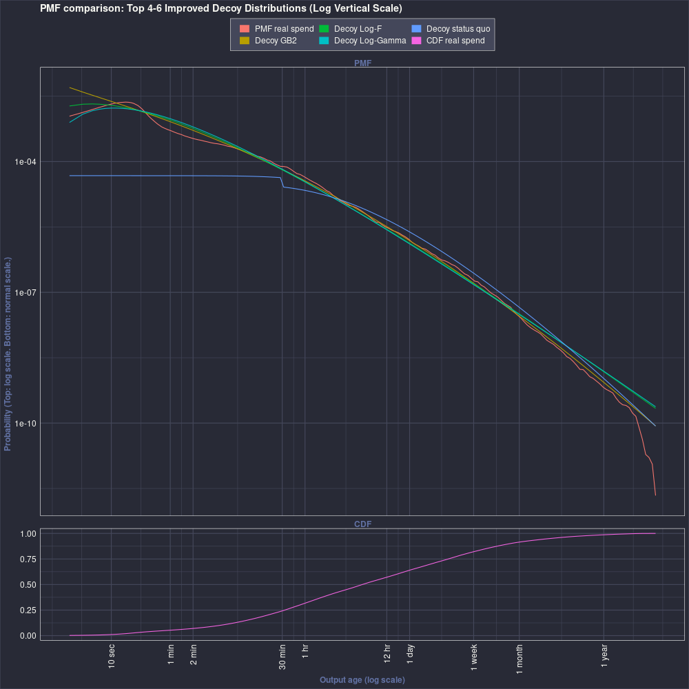
Figure 13.4 is the same plot as Figure 13.2 , except the vertical axis is log scale.

Figure 13.4

13.3 Attack success probability by output age

The MAP decoder attack success probability varies with the age of the spent output. Where the decoy PMF is below the real spend PMF, the attack success probability is high. Where the decoy PMF is above the real spend PMF, the attack success probability is low. Figure 13.5 shows the attack success probability by output age for the top three fitted decoy distributions and the status quo decoy distribution.

There are four regions where the fitted decoy distributions do a poor job of protecting the real spend. The first occurs at about 10-20 seconds of age. As mentioned above, in practice outputs from zero to two minutes of age will be aggregated together, so this region is not of much concern.

The second region is 30 minutes to one hour. Notice that 20 minutes coincides with the “cliff” in the status quo decoy distribution that forms because the unspendable portion of the log-gamma distribution before the 10 block lock is redistributed to the early part of the spendable distribution. The 101-point resolution of the BJR estimator may have had a difficult time with this cliff in the decoy distribution because it is not smooth. The BJR estimator may be overestimating the thickness of the real spend distribution in this region. In other words, this region of high attack success may be a false reading.

The third region extends from the second day to the second week of age.

The fourth region occurs after one year of age. Notice that the log-GB2 and the log-GEV both have high attack success probability in this region, but the RPLN distribution does not. This example shows that the distribution family does affect the regions of the age distribution that would be most susceptible to the MAP Decoder attack, even when the average attack success probability, shown in Table 13.1 , is similar between the distributions. Note also that the CDF shows that the share of rings spending outputs older than one year is very small.

Figure 13.5

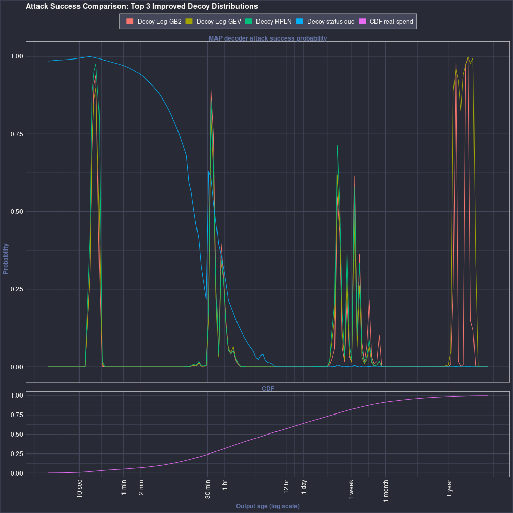
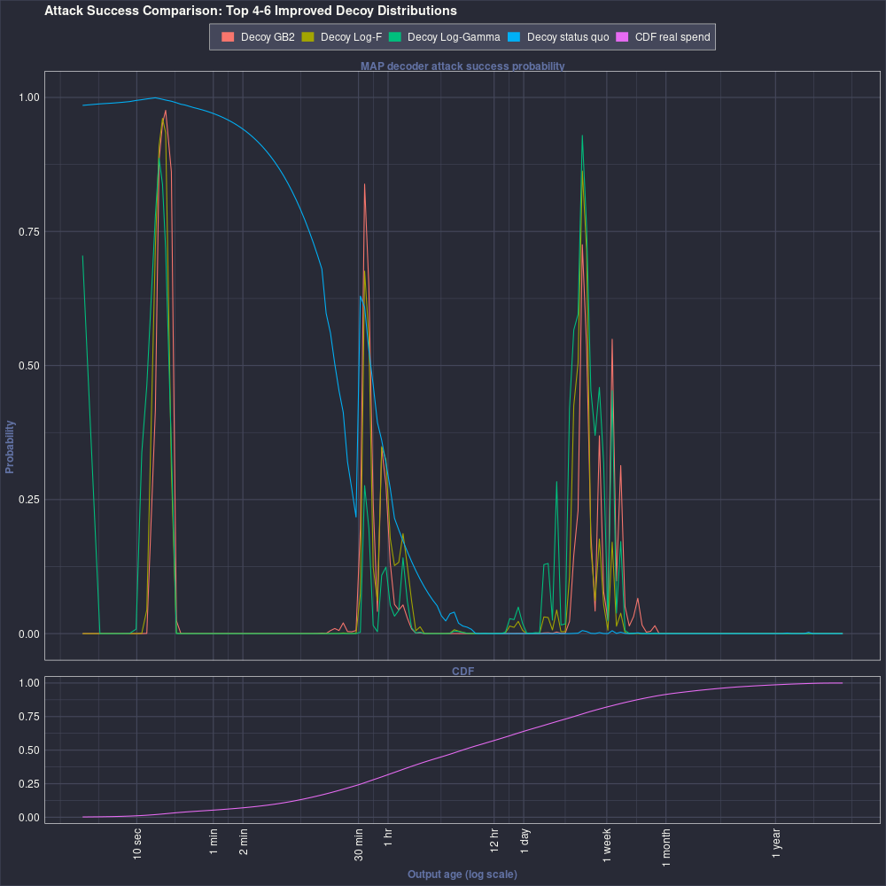
Figure 13.6 shows the same data as Figure 13.5 , except for the top 4-6 fitted distributions.

Figure 13.6

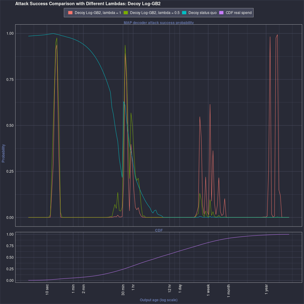
13.4 Attack success probability for different λ weights

We also fitted decoy distributions with different λ weights in Equation 12.2 . The mean attack success probability of these fitted distributions with λ = 0.5 in Table 13.2 are higher than the λ = 1 fitted distributions, which is completely expected. The λ = 0.5 fitted distributions are optimizing to a different objective function, so the value of the λ = 1 objective function is not as good. However, the “loss” of the objective function is not very large, at around 0.2 percentage points for each of them.

Table 13.2: Attack success probability, λ = 1, 0.5

Decoy distribution	λ	Attack success probability	Param 1	Param 2	Param 3	Param 4
Log-GB2	1.0	7.590%	shape1 = 4.462	scale = 20.62	shape2 = 0.5553	shape3 = 7.957
Log-GB2	0.5	7.783%	shape1 = 4.631	scale = 19.76	shape2 = 0.5308	shape3 = 6.235
Log-GEV	1.0	7.730%	location = 8.382	scale = 3.851	shape = -0.3404
Log-GEV	0.5	7.841%	location = 8.608	scale = 3.956	shape = -0.3369
RPLN	1.0	7.746%	shape2 = 6.684	meanlog = 9.725	sdlog = 3.964
RPLN	0.5	7.981%	shape2 = 6.121	meanlog = 9.977	sdlog = 4.064
GB2	1.0	7.794%	shape1 = 0.1282	scale = 4753	shape2 = 8.582	shape3 = 7.179
GB2	0.5	7.984%	shape1 = 0.05374	scale = 8.369e+04	shape2 = 40.93	shape3 = 43.62
Log-F	1.0	8.212%	df1 = 1.678	df2 = 9.067e+06	ncp = 17.06
Log-F	0.5	8.463%	df1 = 1.563	df2 = 3.555e+07	ncp = 16.68
Log-Gamma	1.0	8.470%	shape = 4.315	rate = 0.3751
Log-Gamma	0.5	8.622%	shape = 4.517	rate = 0.3892
Decoy status quo		23.540%	shape = 19.28	rate = 1.61

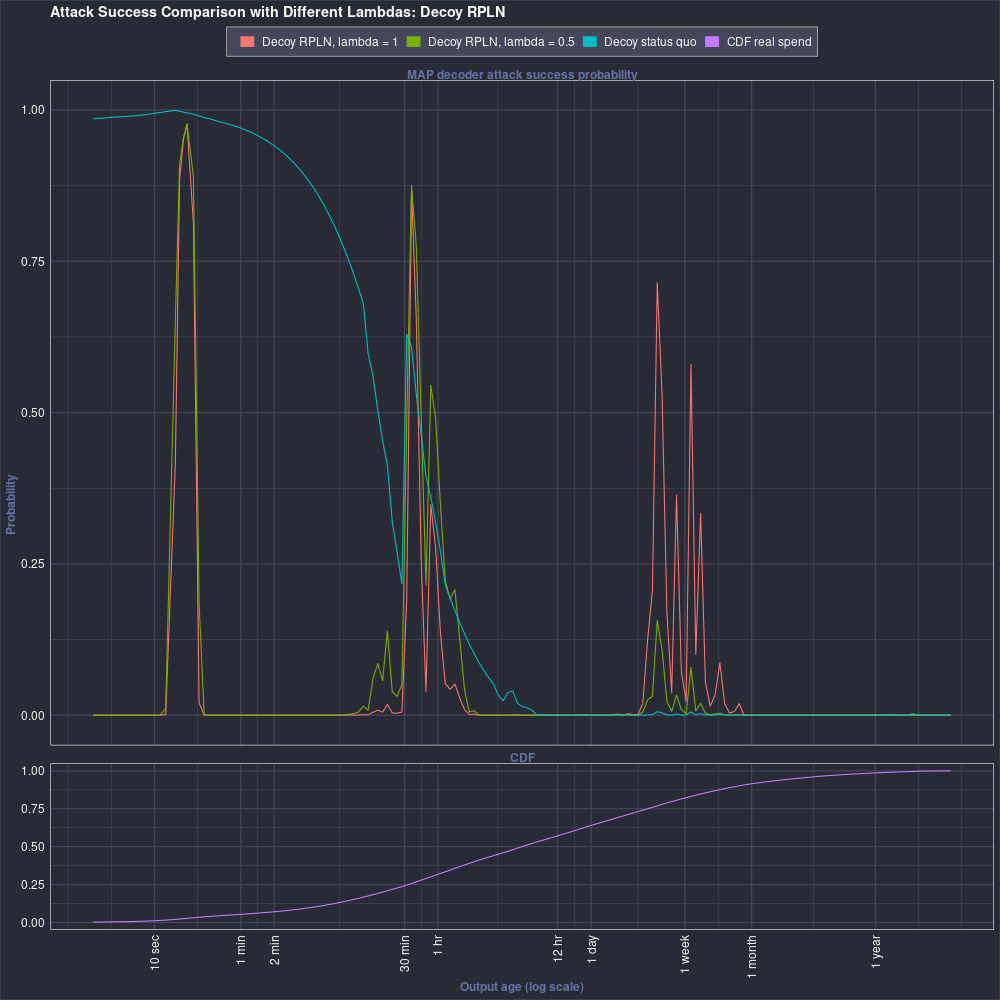
Figure 13.7 shows the attack success probability for the fitted GB2 decoy distributions when λ = 1 and λ = 0.5. One can see that the λ = 0.5 distribution more heavily weights the older outputs, as expected. That distribution has lower attack success probability against the older outputs than the λ = 1 distribution. Of course, the lower attack success probability there comes at the cost of having higher attack success probability against younger outputs.

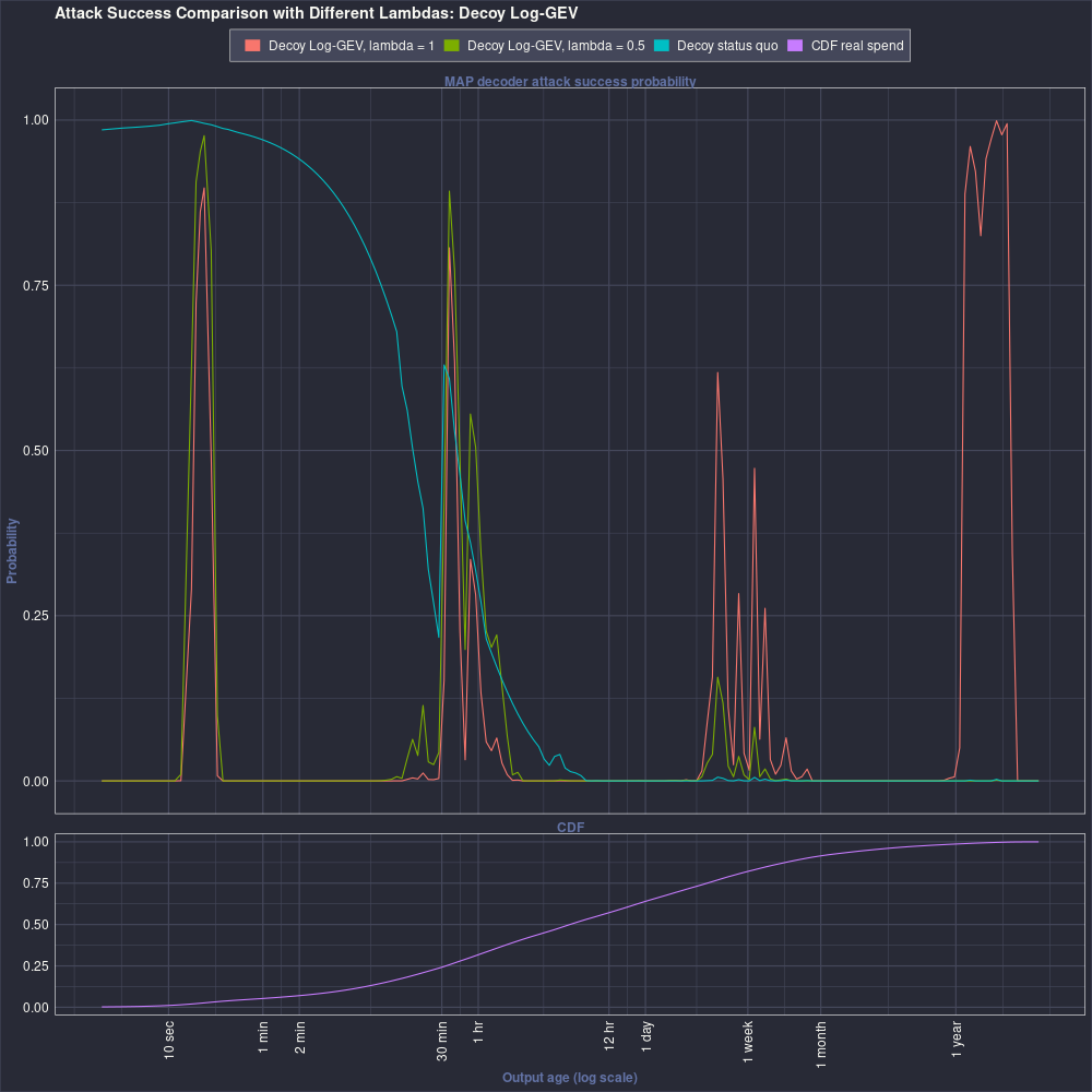
Equivalent plots for the log-GEV and RPLN distribution are in Figure 13.8 and Figure 13.9 .

Figure 13.7

Figure 13.8

Figure 13.9

13.5 Code

library(ggplot2)
library(dRacula)


threads <- 1
# Best to have one thread when do.sub.support == FALSE and when RAM is limited
future::plan(future::multisession(workers = threads))

options(future.globals.maxSize = 8000*1024^2)



# Some of this code could be re-factored to improve categorical selections.


analysis.subset <- order(sapply(fit.results, FUN = function(x) x$value))
analysis.subset <- setdiff(analysis.subset, which(run.iters.simple$lambda != 1))
# Remove results where lambda does not equal 1
analysis.subset <- analysis.subset[1:6]
# Get top 6

analysis.subset.names <- gsub("f_D.", "", names(run.iters.simple$f_D))

analysis.subset.names <- ifelse(analysis.subset.names == "gamma", "Gamma", toupper(analysis.subset.names))
analysis.subset.names[run.iters.simple$log.trans] <- paste0("Log-", analysis.subset.names[run.iters.simple$log.trans])
analysis.subset.names <- analysis.subset.names

low.lambda.subset <- which(run.iters.simple$lambda == 0.5 & 
    analysis.subset.names %in% analysis.subset.names[analysis.subset])

analysis.subset <- c(analysis.subset, low.lambda.subset)
# Add the lambda == 0.5 ones that correspond to the lambda == 1 "best" distributions

analysis.subset <- c(analysis.subset, nrow(run.iters.simple) + 1)
analysis.subset.names <- c(analysis.subset.names, "Decoy status quo")
# Last one is status quo decoy


keep.time <- base::date()


performance.fit.results <- future.apply::future_lapply((1:(nrow(run.iters.simple)+1))[analysis.subset], function(iter) {
  
  GAMMA_SHAPE = 19.28
  GAMMA_RATE = 1.61
  
  G <- function(x) {
    actuar::plgamma(x, shapelog = GAMMA_SHAPE, ratelog = GAMMA_RATE)
  }
  
  G_star <- function(x) {
    (0 <= x*v & x*v <= 1800) *
      (G(x*v + 1200) - G(1200) +
          ( (x*v)/(1800) ) * G(1200)
      )/G(z*v) +
      (1800 < x*v & x*v <= z*v) * G(x*v + 1200)/G(z*v) +
      (z*v < x*v) * 1
  }
  
  
  summary.performance <- data.table(new.decoy = 0)
  
  
  do.sub.support <- FALSE
  
  do.current.decoy <- iter == nrow(run.iters.simple) + 1
  
  guess.prob.each.output <- vector("numeric", z)
  
  
  weekly.z.max <- z
  
  
  theta_i <- aggregate.real.spend.pmf
  
  theta_i[theta_i == 0] <- .Machine$double.eps
  
  if (do.current.decoy) {
    
    if (FALSE) {
      a_i <- aggregate.real.spend.pmf
    } else {
      a_i <- diff(G_star(as.numeric(0:weekly.z.max)))
    }
    
    
    a_i[a_i <= 0] <- .Machine$double.eps
    
    if (do.sub.support) {
      
      set.seed(314)
      sub.supp <- wrswoR::sample_int_expj(length(theta_i), ceiling(length(theta_i)/10), prob = theta_i)
      # start at 2 so G(x - 1) is not 0
      theta_i <- theta_i[sub.supp]
      a_i <- a_i[sub.supp]
    } else {
      sub.supp <- seq_along(theta_i)
    }
    
    stopifnot(length(theta_i) == length(a_i))
    
    values.map.decoder.success.prob <- map.decoder.success.prob(f_S = theta_i/sum(theta_i), f_D = a_i/sum(a_i))
    
    guess.prob.each.output[sub.supp] <- guess.prob.each.output[sub.supp] + values.map.decoder.success.prob
    
    n.decoys <- 15
    
    summary.performance[, new.decoy :=
        sum((theta_i/sum(theta_i)) * (values.map.decoder.success.prob)^n.decoys)]
    
  } else {
    
    f_D.fun <- run.iters.simple$f_D[[iter]]
    fitted.par <- fit.results[[iter]]$par
    log.trans <- run.iters.simple$log.trans[[iter]]
    
    if (do.sub.support) {
      
      set.seed(314)
      sub.supp <- wrswoR::sample_int_expj(length(theta_i), ceiling(length(theta_i)/10), prob = theta_i)
      # start at 2 so G(x - 1) is not 0
      theta_i <- theta_i[sub.supp]
      
    } else {
      sub.supp <- seq_along(theta_i)
    }
    
    
    f_D.return <- f_D.fun(fitted.par, v, z, sub.supp, get.decoy.pmf, log.trans = log.trans)
    
    
    # a_i <- c(f_D.return$decoy.pmf, 0)
    a_i <- f_D.return$decoy.pmf
    
    rm(f_D.return)
    
    a_i[a_i <= 0] <- .Machine$double.eps
    
    
    
    stopifnot(length(theta_i) == length(a_i))
    
    values.map.decoder.success.prob <- map.decoder.success.prob(f_S = theta_i/sum(theta_i), f_D = a_i/sum(a_i))
    
    guess.prob.each.output[sub.supp] <- guess.prob.each.output[sub.supp] + values.map.decoder.success.prob
    
    rm(sub.supp)
    
    n.decoys <- 15
    
    summary.performance[, new.decoy :=
        sum((theta_i/sum(theta_i)) * (values.map.decoder.success.prob)^n.decoys)]
    
  }
  # Note that this code originally iterated through multiple weeks. Some
  # of the design decisions relect that history. 
  
  
  setnames(summary.performance, "new.decoy",
    ifelse(do.current.decoy, "current.decoy", names(run.iters.simple$f_D)[iter]))
  
  list(
    summary.performance = summary.performance,
    decoy.pmf = a_i,
    guess.prob.each.output = guess.prob.each.output/nrow(summary.performance))
  
}, future.globals = c("fit.results", "run.iters.simple", "aggregate.real.spend.pmf",
  "map.decoder.success.prob", "get.decoy.pmf", "v", "z", "actuar::plgamma", "wrswoR::sample_int_expj"),
  future.packages = "data.table", future.seed = TRUE)

print(keep.time)
base::date()


future::plan(future::sequential)
# Stop workers to free RAM
gc()


extracted.params <- lapply(analysis.subset[ - length(analysis.subset)], FUN = function(x) {
  # - length(analysis.subset) to remove the status quo decoy
  deparsed <- paste0(deparse(run.iters.simple$f_D[[x]]), collapse = " ")
  deparsed <- gsub("(.* log.trans, *)|(, *tail.beyond.support.*)|(, lower.tail.*)", "", deparsed)
  deparsed <- gsub(" = [^ ]*", "", deparsed)
  deparsed <- strsplit(deparsed, " ")[[1]]
  deparsed <- deparsed[deparsed != ""]
  
  for (i in seq_along(fit.results[[x]]$par)) {
    param.value <- param.trans[[gsub("f_D.", "", names(run.iters.simple$f_D)[x])]][[i]](fit.results[[x]]$par[i])
    deparsed[i] <- paste0(deparsed[i] , " = ", formatC(param.value, width = 5))
  }
  
  deparsed
  
})

GAMMA_SHAPE = 19.28
GAMMA_RATE = 1.61

extracted.params[[length(extracted.params) + 1]] <-
  c(paste0("shape = ", GAMMA_SHAPE), paste0("rate = ", GAMMA_RATE))

extracted.params <- t(sapply(extracted.params, "length<-", max(lengths(extracted.params))))
# https://stackoverflow.com/questions/15201305/how-to-convert-a-list-consisting-of-vector-of-different-lengths-to-a-usable-data

colnames(extracted.params) <- paste0("Param ", seq_len(ncol(extracted.params)))

n.decoys <- 15

MAP.decoder.effectiveness <- sapply(performance.fit.results, FUN = function(x) {
  sum((aggregate.real.spend.pmf/sum(aggregate.real.spend.pmf)) * (x$guess.prob.each.output)^n.decoys)
})

gc()

MAP.decoder.effectiveness <- data.frame(
  dist.name = analysis.subset.names[analysis.subset],
  MAP.decoder.effectiveness = formatC(MAP.decoder.effectiveness, width = 5))

MAP.decoder.effectiveness <- cbind(MAP.decoder.effectiveness, extracted.params)

MAP.decoder.effectiveness <- as.data.frame(
  lapply(MAP.decoder.effectiveness, FUN = function(x) {x[is.na(x)] <- ""; x} ))

colnames(MAP.decoder.effectiveness)[1:2] <- c("Decoy distribution", "Attack success probability")
colnames(MAP.decoder.effectiveness) <- gsub("[.]", " ", colnames(MAP.decoder.effectiveness))

MAP.decoder.effectiveness$`Attack success probability` <-
  scales::percent(as.numeric(MAP.decoder.effectiveness$`Attack success probability`))

knitr::kable(MAP.decoder.effectiveness[ ! analysis.subset %in% low.lambda.subset, ],
  format = "pipe", row.names = FALSE, digits = 3,
  align = paste0("lr", paste0(rep("l", ncol(extracted.params)), collapse = "")))



MAP.decoder.effectiveness$`λ` <- ifelse(analysis.subset %in% low.lambda.subset, 0.5, 1)

MAP.decoder.effectiveness$`Decoy distribution` <- factor(
  MAP.decoder.effectiveness$`Decoy distribution`,
  levels = c(MAP.decoder.effectiveness$`Decoy distribution`[1:6], "Decoy status quo")
)

MAP.decoder.effectiveness <- MAP.decoder.effectiveness[, c(
  "Decoy distribution", "λ",  "Attack success probability",
  paste0("Param ", seq_len(ncol(extracted.params))) ) ]

knitr::kable(MAP.decoder.effectiveness[
  order(MAP.decoder.effectiveness$`Decoy distribution`,  - MAP.decoder.effectiveness$`λ`), ],
  format = "pipe", row.names = FALSE, digits = 3,
  align = paste0("lrr", paste0(rep("l", ncol(extracted.params)), collapse = "")))





guess.prob.each.output <- performance.fit.results[[1]]$guess.prob.each.output

display.x <- unique(floor(exp(seq(1, 100, by = 0.1))))
display.x <- display.x[display.x <= length(guess.prob.each.output)]
display.x <- display.x[guess.prob.each.output[display.x] != 0]



decoy.plot.data <- lapply(setdiff(analysis.subset, low.lambda.subset), function(x) {
  
  if (x == nrow(run.iters.simple) + 1) {
    
    type <- analysis.subset.names[x]
    
    GAMMA_SHAPE = 19.28
    GAMMA_RATE = 1.61
    
    G <- function(x) {
      actuar::plgamma(x, shapelog = GAMMA_SHAPE, ratelog = GAMMA_RATE)
    }
    
    G_star <- function(x) {
      (0 <= x*v & x*v <= 1800) *
        (G(x*v + 1200) - G(1200) +
            ( (x*v)/(1800) ) * G(1200)
        )/G(z*v) +
        (1800 < x*v & x*v <= z*v) * G(x*v + 1200)/G(z*v) +
        (z*v < x*v) * 1
    }
    
    weekly.z.max <- z
    
    f_D.return <- diff(G_star(as.numeric(0:weekly.z.max)))[display.x]
    
    
  } else {
    type <- paste0("Decoy ", analysis.subset.names[x])
    
    f_D.fun <- run.iters.simple$f_D[[x]]
    fitted.par <- fit.results[[x]]$par
    log.trans <- run.iters.simple$log.trans[[x]]
    
    f_D.return <- f_D.fun(fitted.par, v, z, sub.supp = display.x, get.decoy.pmf, log.trans = log.trans)$decoy.pmf
  }
  
  cat(type, " ", which(x == analysis.subset), " ", x, "\n")
  
  data.frame(x = display.x, y = f_D.return, type = type)
  
})


decoy.plot.data <- rbind(
  do.call(rbind, decoy.plot.data),
  data.frame(x = display.x, y = aggregate.real.spend.pmf[display.x], type = "PMF real spend"),
  data.frame(x = display.x, y = cumsum(aggregate.real.spend.pmf)[display.x], type = "CDF real spend")
)




decoy.plot.data$panel <- ifelse(decoy.plot.data$type == "CDF real spend",
  "CDF", "PMF")

decoy.plot.data$panel <- factor(decoy.plot.data$panel, levels = c("PMF", "CDF"))

decoy.plot.data$type <- factor(decoy.plot.data$type,
  levels = c("PMF real spend", 
    unique(decoy.plot.data$type)[grepl("Decoy", unique(decoy.plot.data$type))],
    "CDF real spend"))


png("images/decoy-distributions-top-1-3-not-log.png", width = 1000, height = 1000)


ggplot(decoy.plot.data[decoy.plot.data$type %in% c("PMF real spend", "CDF real spend",
  "Decoy status quo", paste0("Decoy ", analysis.subset.names[analysis.subset][1:3])), ],
  aes(x = x, y = y, colour = type)) +
  labs( title = "PMF comparison: Top 3 Improved Decoy Distributions",
    y = "Probability",
    x = "Output age (log scale)") +
  geom_line() +
  scale_x_log10(
    guide = guide_axis(angle = 90),
    breaks = c(1/v, 10/v, 60/v, 60*2/v, 60*30/v, 60^2/v, 60^2*12/v, 60^2*24/v, 60^2*24*7/v, 60^2*24*28/v, 60^2*24*365/v),
    labels = c("1 sec", "10 sec", "1 min", "2 min", "30 min", "1 hr", "12 hr", "1 day", "1 week", "1 month", "1 year")) +
  # scale_colour_brewer(palette = "Dark2") +
  ggh4x::facet_manual(facets = vars(panel), design = "A\nB", scale = "free_y", heights = c(8, 2)) +
  guides(linewidth = "none", linetype = "none",
    colour = guide_legend(override.aes = list(linewidth = 5))) +
  ggh4x::facetted_pos_scales(y = list(scale_y_continuous(), scale_y_continuous())) +
  theme_dracula() +
  theme(
    legend.position = "top",
    legend.title = element_blank(),
    panel.border = element_rect(color = "white", fill = NA))
# The order of the themes() matter. Must have theme_dracula() first.

dev.off()


png("images/decoy-distributions-top-4-6-not-log.png", width = 1000, height = 1000)


ggplot(decoy.plot.data[decoy.plot.data$type %in% c("PMF real spend", "CDF real spend",
  "Decoy status quo", paste0("Decoy ", analysis.subset.names[analysis.subset][4:6])), ],
  aes(x = x, y = y, colour = type)) +
  labs( title = "PMF comparison: Top 4-6 Improved Decoy Distributions",
    y = "Probability",
    x = "Output age (log scale)") +
  geom_line() +
  scale_x_log10(
    guide = guide_axis(angle = 90),
    breaks = c(1/v, 10/v, 60/v, 60*2/v, 60*30/v, 60^2/v, 60^2*12/v, 60^2*24/v, 60^2*24*7/v, 60^2*24*28/v, 60^2*24*365/v),
    labels = c("1 sec", "10 sec", "1 min", "2 min", "30 min", "1 hr", "12 hr", "1 day", "1 week", "1 month", "1 year")) +
  # scale_colour_brewer(palette = "Dark2") +
  ggh4x::facet_manual(facets = vars(panel), design = "A\nB", scale = "free_y", heights = c(8, 2)) +
  guides(linewidth = "none", linetype = "none",
    colour = guide_legend(override.aes = list(linewidth = 5))) +
  ggh4x::facetted_pos_scales(y = list(scale_y_continuous(), scale_y_continuous())) +
  theme_dracula() +
  theme(
    legend.position = "top",
    legend.title = element_blank(),
    panel.border = element_rect(color = "white", fill = NA))
# The order of the themes() matter. Must have theme_dracula() first.

dev.off()



png("images/decoy-distributions-top-1-3-log.png", width = 1000, height = 1000)


ggplot(decoy.plot.data[decoy.plot.data$type %in% c("PMF real spend", "CDF real spend",
  "Decoy status quo", paste0("Decoy ", analysis.subset.names[analysis.subset][1:3])), ],
  aes(x = x, y = y, colour = type)) +
  labs( title = "PMF comparison: Top 3 Improved Decoy Distributions (Log Vertical Scale)",
    y = "Probability (Top: log scale. Bottom: normal scale.)",
    x = "Output age (log scale)") +
  geom_line() +
  scale_x_log10(
    guide = guide_axis(angle = 90),
    breaks = c(1/v, 10/v, 60/v, 60*2/v, 60*30/v, 60^2/v, 60^2*12/v, 60^2*24/v, 60^2*24*7/v, 60^2*24*28/v, 60^2*24*365/v),
    labels = c("1 sec", "10 sec", "1 min", "2 min", "30 min", "1 hr", "12 hr", "1 day", "1 week", "1 month", "1 year")) +
  # scale_colour_brewer(palette = "Dark2") +
  ggh4x::facet_manual(facets = vars(panel), design = "A\nB", scale = "free_y", heights = c(8, 2)) +
  guides(linewidth = "none", linetype = "none",
    colour = guide_legend(override.aes = list(linewidth = 5))) +
  ggh4x::facetted_pos_scales(y = list(scale_y_log10(), scale_y_continuous())) +
  theme_dracula() +
  theme(
    legend.position = "top",
    legend.title = element_blank(),
    panel.border = element_rect(color = "white", fill = NA))
# The order of the themes() matter. Must have theme_dracula() first.

dev.off()



png("images/decoy-distributions-top-4-6-log.png", width = 1000, height = 1000)


ggplot(decoy.plot.data[decoy.plot.data$type %in% c("PMF real spend", "CDF real spend",
  "Decoy status quo", paste0("Decoy ", analysis.subset.names[analysis.subset][4:6])), ],
  aes(x = x, y = y, colour = type)) +
  labs( title = "PMF comparison: Top 4-6 Improved Decoy Distributions (Log Vertical Scale)",
    y = "Probability (Top: log scale. Bottom: normal scale.)",
    x = "Output age (log scale)") +
  geom_line() +
  scale_x_log10(
    guide = guide_axis(angle = 90),
    breaks = c(1/v, 10/v, 60/v, 60*2/v, 60*30/v, 60^2/v, 60^2*12/v, 60^2*24/v, 60^2*24*7/v, 60^2*24*28/v, 60^2*24*365/v),
    labels = c("1 sec", "10 sec", "1 min", "2 min", "30 min", "1 hr", "12 hr", "1 day", "1 week", "1 month", "1 year")) +
  # scale_colour_brewer(palette = "Dark2") +
  ggh4x::facet_manual(facets = vars(panel), design = "A\nB", scale = "free_y", heights = c(8, 2)) +
  guides(linewidth = "none", linetype = "none",
    colour = guide_legend(override.aes = list(linewidth = 5))) +
  ggh4x::facetted_pos_scales(y = list(scale_y_log10(), scale_y_continuous())) +
  theme_dracula() +
  theme(
    legend.position = "top",
    legend.title = element_blank(),
    panel.border = element_rect(color = "white", fill = NA))
# The order of the themes() matter. Must have theme_dracula() first.


dev.off()




# Attack success probability


MAP.decoder.plot.data <- lapply(setdiff(analysis.subset, low.lambda.subset), function(x) {
  if (x == nrow(run.iters.simple) + 1) {
    type <- "Decoy status quo"
  } else {
    type <- type <- paste0("Decoy ", analysis.subset.names[x])
  }
  cat(type, " ", which(x == analysis.subset), " ", x, "\n")
  guess.prob.each.output <- performance.fit.results[[which(x == analysis.subset)]]$guess.prob.each.output
  n.decoys <- 15
  data.frame(x = display.x, y = guess.prob.each.output[display.x]^n.decoys, type = type)
})



MAP.decoder.plot.data <- rbind(
  do.call(rbind, MAP.decoder.plot.data),
  data.frame(x = display.x, y = cumsum(aggregate.real.spend.pmf)[display.x], type = "CDF real spend")
)


MAP.decoder.plot.data$type <- gsub("f_D.", "Decoy ", MAP.decoder.plot.data$type)



MAP.decoder.plot.data$panel <- ifelse(MAP.decoder.plot.data$type == "CDF real spend",
  "CDF", "MAP decoder attack success probability")

MAP.decoder.plot.data$panel <- factor(MAP.decoder.plot.data$panel,
  levels = c("MAP decoder attack success probability", "CDF"))

MAP.decoder.plot.data$type <- factor(MAP.decoder.plot.data$type,
  levels = c("PMF real spend", 
    unique(MAP.decoder.plot.data$type)[grepl("Decoy", unique(MAP.decoder.plot.data$type))],
    "CDF real spend"))



png("images/attack-success-top-1-3.png", width = 1000, height = 1000)



ggplot(MAP.decoder.plot.data[MAP.decoder.plot.data$type %in% c("PMF real spend", "CDF real spend",
  "Decoy status quo", paste0("Decoy ", analysis.subset.names[analysis.subset][1:3])), ],
  aes(x = x, y = y, colour = type)) +
  labs( title = "Attack Success Comparison: Top 3 Improved Decoy Distributions",
    y = "Probability",
    x = "Output age (log scale)") +
  geom_line() +
  scale_x_log10(
    guide = guide_axis(angle = 90),
    breaks = c(1/v, 10/v, 60/v, 60*2/v, 60*30/v, 60^2/v, 60^2*12/v, 60^2*24/v, 60^2*24*7/v, 60^2*24*28/v, 60^2*24*365/v),
    labels = c("1 sec", "10 sec", "1 min", "2 min", "30 min", "1 hr", "12 hr", "1 day", "1 week", "1 month", "1 year")) +
  # scale_colour_brewer(palette = "Dark2") +
  ggh4x::facet_manual(facets = vars(panel), design = "A\nB", scale = "free_y", heights = c(8, 2)) +
  guides(linewidth = "none", linetype = "none",
    colour = guide_legend(override.aes = list(linewidth = 5))) +
  ggh4x::facetted_pos_scales(y = list(scale_y_continuous(), scale_y_continuous())) +
  theme_dracula() +
  theme(
    legend.position = "top",
    legend.title = element_blank(),
    panel.border = element_rect(color = "white", fill = NA))
# The order of the themes() matter. Must have theme_dracula() first.


dev.off()



png("images/attack-success-top-4-6.png", width = 1000, height = 1000)


ggplot(MAP.decoder.plot.data[MAP.decoder.plot.data$type %in% c("PMF real spend", "CDF real spend",
  "Decoy status quo", paste0("Decoy ", analysis.subset.names[analysis.subset][4:6])), ],
  aes(x = x, y = y, colour = type)) +
  labs( title = "Attack Success Comparison: Top 4-6 Improved Decoy Distributions",
    y = "Probability",
    x = "Output age (log scale)") +
  geom_line() +
  scale_x_log10(
    guide = guide_axis(angle = 90),
    breaks = c(1/v, 10/v, 60/v, 60*2/v, 60*30/v, 60^2/v, 60^2*12/v, 60^2*24/v, 60^2*24*7/v, 60^2*24*28/v, 60^2*24*365/v),
    labels = c("1 sec", "10 sec", "1 min", "2 min", "30 min", "1 hr", "12 hr", "1 day", "1 week", "1 month", "1 year")) +
  # scale_colour_brewer(palette = "Dark2") +
  ggh4x::facet_manual(facets = vars(panel), design = "A\nB", scale = "free_y", heights = c(8, 2)) +
  guides(linewidth = "none", linetype = "none",
    colour = guide_legend(override.aes = list(linewidth = 5))) +
  ggh4x::facetted_pos_scales(y = list(scale_y_continuous(), scale_y_continuous())) +
  theme_dracula() +
  theme(
    legend.position = "top",
    legend.title = element_blank(),
    panel.border = element_rect(color = "white", fill = NA))
# The order of the themes() matter. Must have theme_dracula() first.


dev.off()








# Compare different lambdas




MAP.decoder.plot.data <- lapply(analysis.subset, function(x) {
  if (x == nrow(run.iters.simple) + 1) {
    type <- "Decoy status quo"
  } else {
    type <- type <- paste0("Decoy ", analysis.subset.names[x])
  }
  cat(type, " ", which(x == analysis.subset), " ", x, "\n")
  guess.prob.each.output <- performance.fit.results[[which(x == analysis.subset)]]$guess.prob.each.output
  n.decoys <- 15
  data.frame(x = display.x, y = guess.prob.each.output[display.x]^n.decoys,
    type = type, lambda = run.iters.simple$lambda[x])
})



MAP.decoder.plot.data <- rbind(
  do.call(rbind, MAP.decoder.plot.data),
  data.frame(x = display.x, y = cumsum(aggregate.real.spend.pmf)[display.x],
    type = "CDF real spend", lambda = 1)
)


MAP.decoder.plot.data$type <- gsub("f_D.", "Decoy ", MAP.decoder.plot.data$type)

MAP.decoder.plot.data$type.reserved <- MAP.decoder.plot.data$type



# Start specific distributions


lambda.distribution <- "Decoy Log-GB2"

MAP.decoder.plot.data$type[MAP.decoder.plot.data$type == lambda.distribution] <- 
  paste0(lambda.distribution, ", lambda = ", 
    MAP.decoder.plot.data$lambda[MAP.decoder.plot.data$type == lambda.distribution])


MAP.decoder.plot.data$panel <- ifelse(MAP.decoder.plot.data$type == "CDF real spend",
  "CDF", "MAP decoder attack success probability")

MAP.decoder.plot.data$panel <- factor(MAP.decoder.plot.data$panel,
  levels = c("MAP decoder attack success probability", "CDF"))

MAP.decoder.plot.data$type <- factor(MAP.decoder.plot.data$type,
  levels = c("PMF real spend", 
    unique(MAP.decoder.plot.data$type)[grepl("Decoy", unique(MAP.decoder.plot.data$type))],
    "CDF real spend"))



png(paste0("images/attack-success-lambda-", tolower(gsub(" ", "-", lambda.distribution)), ".png"),
  width = 1000, height = 1000)


ggplot(MAP.decoder.plot.data[MAP.decoder.plot.data$type %in% c("PMF real spend", "CDF real spend",
  "Decoy status quo") | grepl(lambda.distribution, MAP.decoder.plot.data$type), ],
  aes(x = x, y = y, colour = type)) +
  labs( title = paste0("Attack Success Comparison with Different Lambdas: ", lambda.distribution),
    y = "Probability",
    x = "Output age (log scale)") +
  geom_line() +
  scale_x_log10(
    guide = guide_axis(angle = 90),
    breaks = c(1/v, 10/v, 60/v, 60*2/v, 60*30/v, 60^2/v, 60^2*12/v, 60^2*24/v, 60^2*24*7/v, 60^2*24*28/v, 60^2*24*365/v),
    labels = c("1 sec", "10 sec", "1 min", "2 min", "30 min", "1 hr", "12 hr", "1 day", "1 week", "1 month", "1 year")) +
  # scale_colour_brewer(palette = "Dark2") +
  ggh4x::facet_manual(facets = vars(panel), design = "A\nB", scale = "free_y", heights = c(8, 2)) +
  guides(linewidth = "none", linetype = "none",
    colour = guide_legend(override.aes = list(linewidth = 5))) +
  ggh4x::facetted_pos_scales(y = list(scale_y_continuous(), scale_y_continuous())) +
  theme_dracula() +
  theme(
    legend.position = "top",
    legend.title = element_blank(),
    panel.border = element_rect(color = "white", fill = NA))
# The order of the themes() matter. Must have theme_dracula() first.

dev.off()







lambda.distribution <- "Decoy Log-GEV"

MAP.decoder.plot.data$type <- MAP.decoder.plot.data$type.reserved

MAP.decoder.plot.data$type[MAP.decoder.plot.data$type == lambda.distribution] <- 
  paste0(lambda.distribution, ", lambda = ", 
    MAP.decoder.plot.data$lambda[MAP.decoder.plot.data$type == lambda.distribution])

MAP.decoder.plot.data$type <- factor(MAP.decoder.plot.data$type,
  levels = c("PMF real spend", 
    unique(MAP.decoder.plot.data$type)[grepl("Decoy", unique(MAP.decoder.plot.data$type))],
    "CDF real spend"))



png(paste0("images/attack-success-lambda-", tolower(gsub(" ", "-", lambda.distribution)), ".png"),
  width = 1000, height = 1000)


ggplot(MAP.decoder.plot.data[MAP.decoder.plot.data$type %in% c("PMF real spend", "CDF real spend",
  "Decoy status quo") | grepl(lambda.distribution, MAP.decoder.plot.data$type), ],
  aes(x = x, y = y, colour = type)) +
  labs( title = paste0("Attack Success Comparison with Different Lambdas: ", lambda.distribution),
    y = "Probability",
    x = "Output age (log scale)") +
  geom_line() +
  scale_x_log10(
    guide = guide_axis(angle = 90),
    breaks = c(1/v, 10/v, 60/v, 60*2/v, 60*30/v, 60^2/v, 60^2*12/v, 60^2*24/v, 60^2*24*7/v, 60^2*24*28/v, 60^2*24*365/v),
    labels = c("1 sec", "10 sec", "1 min", "2 min", "30 min", "1 hr", "12 hr", "1 day", "1 week", "1 month", "1 year")) +
  # scale_colour_brewer(palette = "Dark2") +
  ggh4x::facet_manual(facets = vars(panel), design = "A\nB", scale = "free_y", heights = c(8, 2)) +
  guides(linewidth = "none", linetype = "none",
    colour = guide_legend(override.aes = list(linewidth = 5))) +
  ggh4x::facetted_pos_scales(y = list(scale_y_continuous(), scale_y_continuous())) +
  theme_dracula() +
  theme(
    legend.position = "top",
    legend.title = element_blank(),
    panel.border = element_rect(color = "white", fill = NA))
# The order of the themes() matter. Must have theme_dracula() first.

dev.off()






lambda.distribution <- "Decoy RPLN"

MAP.decoder.plot.data$type <- MAP.decoder.plot.data$type.reserved

MAP.decoder.plot.data$type[MAP.decoder.plot.data$type == lambda.distribution] <- 
  paste0(lambda.distribution, ", lambda = ", 
    MAP.decoder.plot.data$lambda[MAP.decoder.plot.data$type == lambda.distribution])

MAP.decoder.plot.data$type <- factor(MAP.decoder.plot.data$type,
  levels = c("PMF real spend", 
    unique(MAP.decoder.plot.data$type)[grepl("Decoy", unique(MAP.decoder.plot.data$type))],
    "CDF real spend"))



png(paste0("images/attack-success-lambda-", tolower(gsub(" ", "-", lambda.distribution)), ".png"),
  width = 1000, height = 1000)


ggplot(MAP.decoder.plot.data[MAP.decoder.plot.data$type %in% c("PMF real spend", "CDF real spend",
  "Decoy status quo") | grepl(lambda.distribution, MAP.decoder.plot.data$type), ],
  aes(x = x, y = y, colour = type)) +
  labs( title = paste0("Attack Success Comparison with Different Lambdas: ", lambda.distribution),
    y = "Probability",
    x = "Output age (log scale)") +
  geom_line() +
  scale_x_log10(
    guide = guide_axis(angle = 90),
    breaks = c(1/v, 10/v, 60/v, 60*2/v, 60*30/v, 60^2/v, 60^2*12/v, 60^2*24/v, 60^2*24*7/v, 60^2*24*28/v, 60^2*24*365/v),
    labels = c("1 sec", "10 sec", "1 min", "2 min", "30 min", "1 hr", "12 hr", "1 day", "1 week", "1 month", "1 year")) +
  # scale_colour_brewer(palette = "Dark2") +
  ggh4x::facet_manual(facets = vars(panel), design = "A\nB", scale = "free_y", heights = c(8, 2)) +
  guides(linewidth = "none", linetype = "none",
    colour = guide_legend(override.aes = list(linewidth = 5))) +
  ggh4x::facetted_pos_scales(y = list(scale_y_continuous(), scale_y_continuous())) +
  theme_dracula() +
  theme(
    legend.position = "top",
    legend.title = element_blank(),
    panel.border = element_rect(color = "white", fill = NA))
# The order of the themes() matter. Must have theme_dracula() first.

dev.off()